Research & Developments is a blog for brief updates that provide context for the flurry of news that impacts science and scientists today.

To date, astronomers have confirmed the existence of just under 6,300 exoplanets. New research could more than double that number, adding a potential 10,000 new planets in one fell swoop.

Yes, that’s right. A 1 with 4 zeros.

The T16 project has announced the discovery of 10,091 exoplanet candidates observed by NASA’s Transiting Exoplanet Survey Satellite (TESS). Since 2018, the all-sky survey has been monitoring more than 200,000 nearby stars using the transit method, which detects the faint dip in a star’s light when a planet crosses in front of it. Astronomers typically require 3 dips to be sure that what they’re seeing is actually a planet and not a one-off event such as an asteroid or comet in that distant star system.

The T16 project analyzed the light curves of more than 54 million stars observed during the first year of the TESS mission. The project’s analysis technique allowed it to search for planets around stars up to 16 times fainter than TESS typically searches, drastically increasing the field of discovery.

Their pipeline detected 11,554 planet candidates. Of those, 1,052 of those had been detected previously and 411 only had one transit—not enough to confirm a planet.

That leaves 10,091 potential new planets. That’s more than were detected in the entirety of NASA’s Kepler mission and its follow-on K2 and more than double the existing planet candidates from TESS that await confirmation. These discoveries will be published in the Astrophysical Journal Supplement.

All of the new planet candidates orbit their stars quickly, with orbital periods between 12 hours and 27 days. Although most of the stars that TESS observes are smaller and cooler than the Sun, those close orbits likely mean that most of those planets are far too hot to be habitable.

The T16 project team confirmed the planet-hood of one of their candidates not using the transit method, but a different method that measures the gravitational tug a planet exerts on its host star. That planet, TIC 183374187, is hot and slightly larger than Jupiter.

The remaining 10,090 newly discovered planet candidates require additional verification to determine whether they truly are planets or not. But given the rigor of the team’s analysis and the requirement of at least 3 transits to even make this list, it’s likely that most of the new discoveries are indeed planets.

“Astronomers are a bit conservative when it comes to claims like this, and want to be sure they pass a bunch of tests to make sure everything was done correctly and these planets actually exist,” astronomer Phil Plait wrote in his Bad Astronomy Newsletter. “Having said that, the process the astronomers went through looks legit to me, and I would bet the majority of these new candidates are real. That’s amazing.”

—Kimberly M. S. Cartier (@astrokimcartier.bsky.social), Staff Writer

These updates are made possible through information from the scientific community. Do you have a story about science or scientists? Send us a tip at eos@agu.org.

Text © 2026. AGU. CC BY-NC-ND 3.0
Except where otherwise noted, images are subject to copyright. Any reuse without express permission from the copyright owner is prohibited.

California is no stranger to the hot, dry summer weather that makes wildfires more likely. But wildfire season in the state is now stretching into the heart of winter, when it has historically been protected by cool, wet weather. In January 2025, Southern California experienced some of the deadliest and costliest wildfires in the state’s history.

Now, a new study published in Nature Communications shows that the climatic changes that increase the risk of these winter wildfires could be driven by low autumn snow levels thousands of miles away, in western Eurasia. The authors said that tracking snowfall in Eurasia could help forecast winters in California that will have higher chances of wildfires.

The researchers were motivated by the catastrophic 2025 wildfires to search for climate drivers of winter wildfire conditions in California. First, they looked for correlations between winter wildfires and ocean temperatures, especially La Niña events that are associated with drier-than-average conditions in California. They also examined variability in sea ice, which can affect global weather patterns. But they saw only weak connections.

Compared to oceans and sea ice, the influence of snow cover on global weather patterns is less studied, said Shineng Hu, a climate scientist at Duke University and lead author of the paper. But another climate researcher in Hu’s lab had previously studied the connection between snow cover and weather patterns and suggested the team look for connections between snow and fires. That’s when they found significant correlations between the winter wildfires in California and low snow cover in western Eurasia.

“When I saw the result, I was suspicious,” Hu said, “because we all know that correlation doesn’t mean causality.” But they ran hundreds of climate model simulations reducing snow cover in Eurasia and saw an increased probability of winter fires in California. “At that point, we were pretty much convinced that there could be something interesting happening over there,” Hu said.

Propagating Pressure

The scientists determined that this intercontinental link starts because the land absorbs more energy when snow cover is low, disturbing the atmosphere above it. This disturbance, like a stone thrown into water, generates large waves of air called Rossby waves that travel eastward along the jet stream across the Pacific Ocean. The Rossby waves drive the formation of a high-pressure zone that creates the hot, dry, windy conditions conducive to wildfires.

“I’m glad to see this group saying snow can do something similar to what ocean temperature anomalies can do,” said Judah Cohen, a climatologist at the Massachusetts Institute of Technology who was not involved in the study but has also studied the links between snow in North America and Eurasia. “I’ve been surprised by how important this mechanism is for U.S. weather in the winter and how little there is about it in the literature.”

But Cohen suggested the study tells only part of the story. In North America, dry winters in the west are paired with wet, cold winters in the east. The same is true in Eurasia, and according to Cohen’s past research, when snow levels are low in western Eurasia but high in eastern Eurasia, a temperature and pressure gradient is created across the continent. The energy released as the atmosphere works to equalize that pressure drives the Rossby waves. Cohen said the disparity between snow levels in eastern and western Eurasia would likely strengthen the Rossby waves and then the warming in California. “If all of Eurasia [had] below normal [snow levels], I don’t think you could easily excite this wave energy that propagates across the hemisphere.” He also stressed that Rossby waves don’t just travel eastward. They also travel upward into the stratosphere, where they bounce back down over North America and intensify the high pressure over the western United States.

Both Cohen and the study authors insisted that many other factors influence whether wildfires ignite in winter. “This is just one missing gap that people didn’t even realize. We want to add that to the table,” said Hu. But monitoring snow levels in Eurasia could offer signs of bad wildfire winters to come. The January 2025 Southern California fires were preceded by low snow levels in November and December in Eurasia, Hu said. “So there’s a 1‑month lag, which gives us some hope that we can use that for prediction.”

—Andrew Chapman (@andrewchapman.bsky.social), Science Writer

Citation: Chapman, A. (2026), Low snow in Eurasia linked to wildfires in California, Eos, 107, https://doi.org/10.1029/2026EO260138. Published on 13 May 2026.

Text © 2026. The authors. CC BY-NC-ND 3.0
Except where otherwise noted, images are subject to copyright. Any reuse without express permission from the copyright owner is prohibited.

For decades, regulators built their ocean monitoring programs mainly around pesticides and pharmaceuticals, treating them as the primary chemical threat to ecological and human health.

That assumption left a much larger category of compounds largely unexamined: the industrial chemicals embedded in packaging, furniture, and everyday personal care products. Those chemicals, it turns out, have been spreading widely. And they’re now showing up even in the places some might consider pristine, such as coral reefs in the Caribbean.

These compounds are biologically active, some interfere with microbial metabolism, and according to a sweeping meta-analysis published in Nature Geoscience, they may be altering how the ocean cycles carbon, one of our planet’s most critical biogeochemical processes.

“Beyond the usual [pesticides and pharmaceuticals], what really surprised us was that everyday industrial chemicals are showing up at even higher levels and not just in coastal or polluted areas, but pretty much everywhere,” said Daniel Petras, a biochemist at the University of California, Riverside.

Led by Petras and Jarmo-Charles Kalinski, a postdoctoral fellow at the Rhodes University Biotechnology Innovation Centre, the study reanalyzed 21 publicly available datasets comprising seawater samples collected over more than a decade across the Pacific, Indian, and North Atlantic Oceans, including the Baltic and Caribbean Seas.

All groups the researchers examined—industrial pollutants, pharmaceuticals, and pesticides—belong to a class called xenobiotics: human-made organic compounds that are foreign to natural systems. Pesticides and pharmaceuticals were prevalent in coastal samples, as expected, given their well-documented entry through agricultural runoff and wastewater outfalls.

But industrial compounds behaved differently. Polyalkylene glycols used in hydraulic fluids, phthalates from polyvinal chloride (PVC) packaging, organophosphate flame retardants from furniture and electronics, and surfactants from personal care products proved far more widespread across all ecosystem types than either pesticides or pharmaceuticals. “These are chemicals we use all the time,” Petras said, “so they end up spreading widely.”

Glimpsing What Was Always There

To map the ocean’s full chemical landscape, the researchers analyzed more than 2,300 samples from temperate coastal zones, coral reefs, and the open ocean, searching for the presence of xenobiotics and examining the share of dissolved organic matter (DOM), a pool of carbon-containing molecules dissolved in seawater. In total, the team identified 248 known xenobiotic molecules. Their work offers the most comprehensive chemical map of anthropogenic organic pollution in the ocean to date.

Researchers used nontargeted mass spectrometry paired with scalable computational tools. Unlike conventional targeted analysis, which tests only for a predefined list of known hazardous molecules, this open-ended approach can detect thousands of chemicals simultaneously, even at low concentrations. The team then applied molecular networking, a computational technique that enables the identification of not only known substances but also their “families” or derivatives.

Coral Reefs as Far-Flung Hot Spots

For Petras, it was surprising to find these compounds in coral reefs like those in French Polynesia, which are typically viewed as perfect, “postcard-style” paradises. Yet closer examination reveals that these areas are, indeed, rarely isolated. Agriculture, urban runoff, hotel infrastructure, and cruise ship traffic all contribute pollutants. Remnants of human activity, such as sunscreen, wastewater, and boat fluids, are concentrated near reefs.

“We specifically detected plasticizers and flame retardants even in these remote areas,” Petras said. “This suggests that our traditional idea of ‘pristine’ needs a serious rethink, as anthropogenic potential sources are now present nearly everywhere.”

Anastazia T. Banaszak, a researcher at the Reef Systems Unit of the Universidad Nacional Autónoma de México who was not involved in the study, stressed the broader implications for reef conservation: “Inadequately treated urban wastewater discharges pose a risk to coral reefs and the success of restoration projects,” she said. Such discharges raise nutrient levels, fueling macroalgal blooms that grow faster than corals and compete with them for space. This pressure on ecosystems is intensifying as climate change shifts the baseline against which restoration outcomes are measured, Banaszak noted.

Carbon…and Microbes?

Beyond reefs, these synthetic compounds could be affecting the ocean’s carbon cycle. DOM is one of Earth’s largest carbon reservoirs, comparable in size to all the carbon dioxide (CO₂) in the atmosphere. Marine microbes transform it from readily degradable forms into biologically resistant ones; refractory DOM that escapes microbial consumption accumulates in the ocean and acts as an important climate regulator.

But with industrial compounds representing up to 63% of DOM in some estuarine samples (with a global estimate of 10%), the microbial loop is, perhaps, facing chemical conditions it did not evolve to handle. This shift means the efficiency of the ocean’s carbon pump, the mechanism that pulls CO₂ from the atmosphere, could be compromised in ways that are not yet understood.

“The data suggest they are present at substantial levels,” Petras said. “Enough that they should be considered in models of carbon cycling.”

Handling the Invisible

Finding xenobiotics is only the first step, the authors say. They laid out several suggestions for next steps. For instance, governments should mandate open-ended approaches as a standard monitoring tool, not just targeted testing of preselected chemicals. Oceanographic data also should be publicly available and standardized, following FAIR (findable, accessible, interoperable, reusable) principles.

“There’s already a strong track record of building long-term datasets for things like trace metals and nutrients. I hope that nontargeted analysis could become part of such long-term efforts,” Petras concluded. “We’ve been quite active in establishing these tools for the community.”

—Mariana Mastache-Maldonado (@deerenoir.bsky.social), Science Writer

Citation: Mastache-Maldonado, M. (2026), Have we been focusing on the wrong ocean pollutants? This study maps what we’ve been missing, Eos, 107, https://doi.org/10.1029/2026EO260151. Published on 13 May 2026.

Text © 2026. The authors. CC BY-NC-ND 3.0
Except where otherwise noted, images are subject to copyright. Any reuse without express permission from the copyright owner is prohibited.

Editors’ Vox is a blog from AGU’s Publications Department.

Ensuring the sustainability of water resources and ecosystems in a changing world requires a thorough understanding of how water moves through Earth’s Critical Zone, a dynamic interface where air, water, soil, plants, and rocks interact. Researchers can track and model this movement of water using naturally occurring markers or “tracers.”

A recent article in Reviews of Geophysics explores the latest advancements in tracer-aided mixing models and how they can help us to better understand the Critical Zone. Here, we asked the authors to give an overview of the Critical Zone, how tracer-aided mixing modeling works, and future directions for research.

What is the Critical Zone (CZ)?

The Critical Zone is Earth’s “living skin”—the dynamic layer where the atmosphere, hydrosphere, biosphere, and lithosphere interact. It stretches from the top of the vegetation canopy and, in cold regions, from the surface of snowpacks and glaciers, down through soils and into the deeper aquifers. It encompasses lakes, streams, and wetlands at the surface, and extends beyond the soil layer to underlying groundwater aquifers. It is where rainfall, snowmelt and glacier melt become soil moisture, where plants take up water and return it to the atmosphere, where aquifers get recharged, and where streamflow is generated. In short, the Critical Zone is where most processes that sustain terrestrial life and freshwater resources unfold.

Why is it important to understand how water moves through the Critical Zone?

Virtually every freshwater resource we rely on (e.g., drinking water, irrigation) passes through the Critical Zone at some point. Global warming, land-use changes, and intensifying water demand emerging from rapid urbanization and changes in agriculture are reshaping how water is stored and released within the Critical Zone, often in ways we cannot yet predict. Understanding how much water is stored within the Critical Zone, how this water is both recharged from rainfall and snowmelt and eventually discharged into streams, and the timescale of these dynamic processes is essential for protecting ecosystems, safeguarding water supplies, and adapting to a changing climate.

How would you explain a tracer-aided mixing model to a non-specialist?

Imagine mixing a glass of orange juice with a glass of apple juice, and trying afterwards to work out how much of each went into the glass. If the juices had distinctive “fingerprints” (imagine its color, sugar content, or a specific chemical) and these fingerprints primarily changed because of the mixing of these two juices, you can then measure the fingerprint in the final mixture and back-calculate the proportion of its distinct sources.

Tracer-aided mixing models work in a similar way but can track the entire water cycle. Different water sources (e.g., rainfall, snowmelt, glacier melt, soil water, groundwater) can have distinct “fingerprints” in a naturally occurring tracer, such as stable isotopes of water or specific dissolved elements. By measuring these fingerprints in the streamwater or groundwater and in its potential sources for example, hydrologists can estimate how much each source contributed to the streamwater or groundwater.

What are some of the most significant and exciting recent advances in tracer-aided mixing models?

Classical mixing models relied on demanding assumptions: that all water sources can be identified and sampled, and that their signatures were distinct and constant in time. Much of the recent progress has been about relaxing these assumptions.

Bayesian approaches now estimate full probability distributions and provide a more realistic picture of uncertainty. Methods like Convex Hull End-Member Mixing Analysis (CHEMMA) use machine learning to infer the distinct sources directly from data, while ensemble hydrograph separation exploits tracer fluctuations over time, thereby making un-mixing feasible even when multiple sources have overlapping signatures. Perhaps the most conceptually novel advance is end-member splitting, which flips the question from “where does streamflow come from?” to “where does precipitation go?”

Alongside these modeling advances, there have been immense advances in how tracers are measured. Portable laser and mass spectrometers now enable high-frequency, in-situ tracer measurements which allows us to capture critical hydrological events such as storms and snowmelt in near-real time.

What are stable water isotope tracers and what are their advantages?

Stable water isotopes are naturally occurring non-radioactive atoms of hydrogen and oxygen that make up a water molecule but have slightly different molecular masses. The two stable isotopes widely used in hydrology are 2H (deuterium) and 18O (oxygen-18). Because these isotopes are part of the water molecule itself, they directly travel with the water molecule. Their key advantages are: (1) they are conservative, meaning they do not react chemically as water moves through soils and aquifers, and (2) they carry distinct signatures resulting from climatic variables such as air temperature.

Consequently, in the European Alps, winter precipitation has a different isotopic signature than summer precipitation because winters are cooler than summers. Other hydrological processes such as evaporation and sublimation leave a recognizable fingerprint on the remaining water, thereby allowing us to estimate how much evaporation or sublimation occurred. Stable water isotopes can be measured in essentially every water compartment, from atmospheric vapor and precipitation to snowpack, plant xylem, soil water, streams, and groundwater. Together, these properties make stable water isotopes the most versatile and widely used tracer in Critical Zone hydrology.

What are the current limitations of tracer-aided mixing models?

Despite their power, mixing models still face many constraints. End-member signatures vary in space and time, are sometimes too similar to distinguish, and some sources may be overlooked entirely. Non-conservative tracers such as nitrate or sulfate can react with their environment along their journey, thereby biasing results if these reactions are not explicitly accounted for.

Sampling is another major bottleneck. Capturing the spatial heterogeneity of soils, snowpacks, and groundwater requires a lot of measurements that are often logistically or financially prohibitive, especially in remote regions. Many of the newer, more powerful tracers such as noble gases or stable isotopes of trace elements, can only be analyzed by a handful of specialized laboratories. As a result, global coverage remains highly uneven, with key regions such as the Arctic and the global South still under-sampled.

What are some of the major unsolved questions and where is more research needed?

There are several fronts where more research is needed. Source signatures are not static, and methods that explicitly capture their variability in time are still underdeveloped. Embedding tracers within global Earth System Models would, in theory, enable more accurate assessment of hydrological partitioning e.g., how rainfall, snowmelt, and glacier melt are split between sublimation, evapotranspiration, groundwater, and streamflow. These will directly inform more robust climate projections, but this remains technically demanding.

Expanding data coverage in under-sampled regions is critical, and citizen science and low-cost sensors may help. Machine learning is a promising approach for uncovering non-linear relationships and gap-filling sparse datasets, but requires training data that often do not yet exist. Greater interdisciplinary integration, e.g., combining tracers with remote sensing, ecological indicators, and biogeochemical data, could yield a more holistic view of the Critical Zone. Finally, the field would benefit from shared protocols and open data practices to enhance progress.

—Andrea L. Popp (andrea.popp@smhi.se; 0000-0003-3911-8105), Swedish Meteorological and Hydrological Institute, Sweden; Harsh Beria (hberia@ethz.ch; 0000-0003-2597-9449), ETH Zurich, Switzerland

Editor’s Note: It is the policy of AGU Publications to invite the authors of articles published in Reviews of Geophysics to write a summary for Eos Editors’ Vox.

Citation: Popp, A. L., and H. Beria (2026), Tracing water’s hidden journey through the Earth’s living skin, Eos, 107, https://doi.org/10.1029/2026EO265019. Published on 13 May 2026.

This article does not represent the opinion of AGU, Eos, or any of its affiliates. It is solely the opinion of the author(s).

Text © 2026. The authors. CC BY-NC-ND 3.0
Except where otherwise noted, images are subject to copyright. Any reuse without express permission from the copyright owner is prohibited.

Research & Developments is a blog for brief updates that provide context for the flurry of news that impacts science and scientists today.

Sand is the most exploited solid natural resource on Earth. It has been integrated into how we build homes, roads, buildings, and bridges as well as how we protect coastal infrastructure from rising seas. Sand underpins nearly every aspect of modern infrastructure and economics, plays crucial roles in supporting ecosystem biodiversity, and literally shores up rivers and coasts.

A new report from the United Nations Environment Programme (UNEP) found that we are using 50 billion metric tons (50 trillion kilograms) of sand per year. As global development and industrialization expand, demand for sand in the building sector is expected to rise 45% by the year 2060, outpacing current efforts to sustainably harvest it. The report’s authors urge countries to establish sand as a strategic national asset and develop policies for sustainable extraction.

“Sand is sometimes referred as the unrecognized hero of development, but its essential role in sustaining the natural services on which we depend is even more overlooked,” Pascal Peduzzi, director of the UNEP Global Resource Information Database Geneva, said in a press release about the report. “Sand is our first line of defence against sea level rise, storm surges, and salination of coastal aquifers—all hazards exacerbated by climate change.”

Sand Wanted: Dead or Alive

Dead sand, or sand that has been extracted from its natural environment, is a key component in building materials like concrete and asphalt. Communities around the world use sand in water filtration systems, providing clean water for drinking and agricultural use. And although a transition to clean energy sources is necessary to curb the effects of climate change, many of those sources also depend on sand: solar panels require glass made from high-purity silica sand, and wind turbines, hydroelectric dams, and nuclear power plants all require concrete.

Sand also plays a critical role in natural ecosystems. It is home to a wide array of critters from crabs, sharks, and turtles to microorganisms like bacteria and fungi. It supports the growth of corals, mangroves, and seagrasses that in turn support even more marine creatures. It is a key component of healthy soil and aids in surface drainage. It guides river evolution and acts as flood buffer and storm barrier. It also provides local economic benefits via tourism.

These are among the values of sand when it is left alone and unused, called “alive” sand. The UN report notes that these benefits are typically of greater value over time than if sand is dredged and used. But because these benefits are hard to see, they are often overlooked when nations calculate the value of their sand resources.

A Sustainable Sand Future

Despite sand’s importance whether dead or alive, the report notes that few countries have established sand as a strategic national asset or have developed strategies for sustainable extraction. At the current pace, humans are extracting sand from the natural environment at a faster pace than it is being replenished by geologic processes.

What’s more, the UNEP’s Marine Sand Watch tool shows that about half of sand dredging companies are operating within marine protected areas, accounting for about 15% of the volume of dredged sand. This practice, the report notes, is potentially trading in sand’s long-term benefits for short-term gains.

The UN report recommends a few actions to protect the long-term availability of sand as a natural resource, including:

• Recognizing sand as strategic national asset, establishing national inventories, and creating long-term regional planning groups that consider sand as an essential resource for resilience;
• Establishing circularity and recycling of building materials, especially in areas of conflict and natural disasters;
• Strengthening environmental protection practices, and codifying international frameworks to strengthen accountability along the supply chain, including increased transparency about extraction; and
• Integrating sand-related biodiversity and social risks into financial decisionmaking and governance.

“Over-reliance on short-term economic metrics risks obscuring, and further impacting, the geological and ecological processes that take centuries to form and may not be restored once critical thresholds are crossed,” the report states. “What is hardest to measure may be precisely what sustains both nature and human societies over the long term. The challenge ahead is not only to manage extraction, but to recognise and balance the full spectrum of sand’s values.”

—Kimberly M. S. Cartier (@astrokimcartier.bsky.social), Staff Writer

These updates are made possible through information from the scientific community. Do you have a story about science or scientists? Send us a tip at eos@agu.org.

Text © 2026. AGU. CC BY-NC-ND 3.0
Except where otherwise noted, images are subject to copyright. Any reuse without express permission from the copyright owner is prohibited.

This migration can be seen in these images of Canada’s Waterton Lakes National Park…

…and of Jackson Glacier in Montana’s Glacier National Park, for example.

But new research, published in the International Journal of Applied Earth Observation and Geoinformation, paints a more complicated picture: Between 2000 and 2020, 42% of tree lines shifted up, true. But 25% of them actually moved downhill.

Sabine Rumpf, an ecologist at the University of Basel in Switzerland, said many studies of tree line shifts tend to be concentrated in limited geographic areas. A preponderance are based primarily on data from North America, Europe, and the Himalayas, where researchers are more likely to have funding to head to the field to take measurements themselves.

“But that also means that a large proportion of the surface of our planet is so understudied,” Rumpf said. “And [to remedy] that, remote sensing data [are] really amazing because you can get a truly global picture, even though there’s nobody, or too few people, observing things in the field.”

Tree Lines Aren’t Living up to Their Potential

So the team set out to take a more global look. They used a world mountain map, developed in 2018, with a 250-meter resolution. They did exclude some regions from their analysis: cells with less than 10% high-mountain coverage (which have so few trees that they don’t have much of a tree line) and cells more than 95% covered with trees (which have so many trees that they don’t have much of a tree line). For their purposes, the team defined the “observed tree line” as the upper limit of trees that stand 3 meters or taller.

Then, said Rumpf, they used a model to calculate the potential tree lines for each area, because, thanks to human effects on the environment, “where these trees could be surviving is almost always higher than where the trees are currently.” The model looked at the growing season length and mean growing season temperature for each cell in the map’s grid. The researchers determined that if a cell had a growing season length of 94 days or longer, and an average growing season temperature of 6.4°C or higher, it could potentially host trees. Cells that didn’t meet both criteria were considered unable to be covered in forest, and thus above the potential tree line.

Jordon Tourville, a terrestrial ecologist with the Appalachian Mountain Club, said the overall findings are not surprising, because other studies have shown seemingly “paradoxical downslope shifts in some cases.” But he noted that whereas this study estimated potential tree lines based on temperature constraints, some scientists have suggested that factors such as nutrient availability and wind exposure are also important in determining tree line position.

Unsurprising, on Second Thought

Armed with this information about observed versus potential tree lines, the researchers hypothesized that areas with the smallest deviation between the two were mostly responding to climatic factors. In contrast, they speculated, areas with a greater difference between observed and potential tree lines were likely experiencing more anthropogenic disturbance, such as logging, agriculture, and infrastructure development.

Their hypothesis held up. In areas with less human disturbance, tree lines were moving upward more quickly (the researchers noted, though, that the upward migration of tree lines lagged behind the rate of climate change). In areas with more human disturbance, the upward spread of trees is suppressed, or even reversed.

Rumpf and several of her colleagues are located in the Alps, where glaciers are retreating, tree lines are climbing, and towns are generally more threatened by mudslides than by wildfires.

Some of the study’s findings, like a quarter of tree lines shifting down, or such a clear signal from wildfires in some areas, were at first unexpected. But after some reflection, Rumpf realized the diversity of data was a perfect example of why global-scale research is important.

“A lot of scientific funding is based in North America and Europe,” Rumpf said, which means many studies return similar results. “Then we do something global and we are surprised that things are different somewhere else on the globe?… I mean, well, duh.”

—Emily Gardner (@emfurd.bsky.social), Associate Editor

This news article is included in our ENGAGE resource for educators seeking science news for their classroom lessons. Browse all ENGAGE articles, and share with your fellow educators how you integrated the article into an activity in the comments section below.

Citation: Gardner, E. (2026), Tree lines are migrating. Some up, some down., Eos, 107, https://doi.org/10.1029/2026EO260146. Published on 12 May 2026.

Text © 2026. The authors. CC BY-NC-ND 3.0
Except where otherwise noted, images are subject to copyright. Any reuse without express permission from the copyright owner is prohibited.

For roughly 45 million years, the eastern section of the African continental plate has been slowly pulling apart. Like a giant zipper extending from the Red Sea to Mozambique, the East African Rift System will likely be home to new oceanic crust that will well up from the widening split in Earth’s surface. While most of the rifts in that system are still zipped shut, the Afar region in northern Ethiopia has already partially unzipped and may be starting to create a future ocean basin.

Most models of this rift system suggest that it should continue to unzip sequentially from north to south. However, new research suggests that a region in the middle of the zipper is on the verge of splitting open.

High-resolution seismic reflection data show that the crust near Kenya’s Lake Turkana is only 13 kilometers thick. This suggests that the region has entered the second stage of rifting, called necking, and is one step closer to breaking apart. It is the only rift zone on Earth currently undergoing this short-lived tectonic process.

Breaking Up Is Hard to Do

Just like mid-ocean ridges on the seafloor, sections of Earth’s crust on land also stretch apart as tectonic plates separate. This process, called rifting, takes place in three stages. First, the crust stretches, creating tension. Then it rapidly thins like pulled taffy—this is the necking stage. Finally, magma wells up from the lithospheric mantle, which creates new seafloor and breaks the continental plate apart.

Not every rift makes it that far. Some remain stuck in the stretching phase with crust more than 20 kilometers thick. But northern sections of the East African Rift System (EARS), specifically the Afar Rift and the Red Sea, are already undergoing the final stage, oceanization.

“This is one of the unique places on Earth where you can see a continental rift,” said Anne Bécel, a geophysicist at Lamont-Doherty Earth Observatory of Columbia University in Palisades, N.Y., and coauthor of new research published in Nature Communications in April. “The East African Rift System has been studied for a very long time by geologists to really learn about our planet and how continents break apart, and then transpose that to mid-ocean ridges where oceanic plates spread apart.”

The team suspected that the Turkana Rift Zone, located at a critical triple junction in northern Kenya, was behaving differently from other areas of the rift system. It is home to an unusually large and continuous hominin fossil record dating back about 4 million years. Past research has also shown that the bottom of the crust, called the Moho, is unusually shallow in the Turkana Basin, just 20 kilometers deep compared with the average depth of 39 kilometers farther away from the rift.

During several field expeditions to Lake Turkana in partnership with local industries, the team mapped the top of the continental crust using borehole measurements and seismic reflection—sending seismic waves into the ground and measuring how the waves bounce back, like sonar. They combined those measurements with past research into Moho depths to calculate the crustal thickness near Lake Turkana.

That map showed that far away from the rift, the crust is more than 35 kilometers thick, but in the Turkana Rift Zone it is a mere 13 kilometers thick, below the threshold for necking.

“If you look at the modern day topography, the whole East African Rift is in this really low, broad land between two big plateaus, one to the north in Ethiopia and one towards the south,” said lead researcher Christian Rowan, a geologist and doctoral candidate at Columbia University. “It’s this very strange topographic feature, and part of that low-lying topography is actually how thin the crust is there.”

“The oldest rocks that record the initiation of the East Africa Rift System are also in the Turkana Rift,” said coauthor Folarin Kolawole, a Columbia University geologist. Geochemical analysis of those rocks suggests that necking in the Turkana Rift Zone began about 4 million years ago.

About to Break?

“Any time you have a place on the planet that is rare in the modern but seen in the past, it is compelling,” said Erik Klemetti Gonzalez, a volcanologist at Denison University in Granville, Ohio, who was not involved with this research. “The data does show that the Turkana Rift is the home of anomalously thin continental crust, so if you are looking for a location that meets criteria for necking, it seems to be the case.”

The team suspects that Turkana might have been primed to split apart more easily because another rifting event took place there a mere 17 million years before the present rift began. The Turkana Basin inherited a weaker section of crust that didn’t have time to fully heal in the (geologically) short time between rifting events. There was also an extended period of magmatic activity throughout much of the past 45 million years.

“Magmatism is well known to be a significant weakening factor in rifting,” Rowan said. “I think the two compounding effects of this inheritance and then magnetism is why the Turkana rift is so much more mature than other segments.”

“There are many ‘failed rifts’ in the geologic record, so the question of whether the EARS is actually leading to a continental break up, albeit a small one, is still very much up in the air,” Klemetti Gonzalez said. These new results tip the scales toward breakup, but he noted that more of the rift system still needs to be mapped to really understand the fate of this region.

“I would hope that more collaboration with African geoscientists could create the ability to collect data from places that have been more inaccessible over the past half century,” he added.

Rowan and his team are working toward that end by continuing to map crustal thicknesses in other nearby rift zones.

“This was the only known rift that was undergoing necking along the entire East African Rift System, or in the world,” said Kolawole. “But based on ongoing work, there is evidence that there are other segments that are at the onset of necking in the East African Rift System.”

—Kimberly M. S. Cartier (@astrokimcartier.bsky.social), Staff Writer

Citation: Cartier, K. M. S. (2026), Eastern Africa is splitting apart, but not where we expected, Eos, 107, https://doi.org/10.1029/2026EO260148. Published on 12 May 2026.

Text © 2026. AGU. CC BY-NC-ND 3.0
Except where otherwise noted, images are subject to copyright. Any reuse without express permission from the copyright owner is prohibited.

Research & Developments is a blog for brief updates that provide context for the flurry of news that impacts science and scientists today.

As the midpoint of the year approaches, several climate records have already been broken. Arctic winter sea ice extent reached a record low. Several countries saw record-breaking winter heat waves. And more than 150 million hectares have already burned globally in wildfires. 

The increasingly likely emergence of an El Niño this summer will likely continue the year’s record-breaking weather trends and could lead to “an unprecedented year of global fire,” according to a statement from World Weather Attribution, a climate research collaboration. 

NOAA’s Climate Prediction Center predicts there is a 61% chance of El Niño—a natural climate pattern that involves warming waters in the Pacific Ocean—emerging by July 2026 and persisting through the end of the year. El Niño typically temporarily boosts global temperatures. 

At a press briefing on 11 May hosted by World Weather Attribution, climate scientists outlined the potential risks of this emerging El Niño against the backdrop of human-caused climate change, including intensifying wildfire seasons, extreme heat waves, and worsening droughts.

In the press briefing, Frederike Otto, a climate scientist at World Weather Attribution and Imperial College London, emphasized that climate change will likely play a larger role in the rest of this year’s extreme weather events than El Niño will, pointing to more than 100 analyses done by World Weather Attribution that have controlled for the effects of the El Niño Southern Oscillation (ENSO), the broader climate phenomenon that produces El Niño and its sister condition, La Niña. 

“We find that human-induced climate change has a much greater influence on the likelihood and intensity of extreme weather events than ENSO,” she said. 

Still, El Niño could push average global temperatures to extremes. The effects of El Niño will “be amplified considerably by the now nearly 1.5°C [(2.7°F)] of global warming experienced as of 2026,” Daniel Swain, a climate scientist at the University of California, Los Angeles and the California Institute for Water Resources, said in a statement. “In modern human history, we’ve never experienced a strong or very strong El Niño event amid pre-existing conditions that were this warm globally.”

The global fire season has “got off to a very fast start,” particularly in the African savanna, Southeast Asia, and northeastern China, Theodore Keeping, who studies extreme weather and wildfires at Imperial College London and World Weather Attribution, said in the briefing. Though El Niño may have mixed effects on the U.S. wildfire season, much of the U.S. is expected to face elevated wildfire risk, and a strong El Niño could worsen wildfires elsewhere in the world, particularly in the Amazon rainforest and Australia, Keeping said. 

“This rapid start [to the wildfire season], in combination with the forecast El Niño, means that we’re looking at a particularly severe year materializing,” Keeping said. “The likelihood of harmful, extreme fires potentially could be the highest we’ve seen in recent history.”

—Grace van Deelen (@gvd.bsky.social), Staff Writer

These updates are made possible through information from the scientific community. Do you have a story about science or scientists? Send us a tip at eos@agu.org.

Text © 2026. AGU. CC BY-NC-ND 3.0
Except where otherwise noted, images are subject to copyright. Any reuse without express permission from the copyright owner is prohibited.

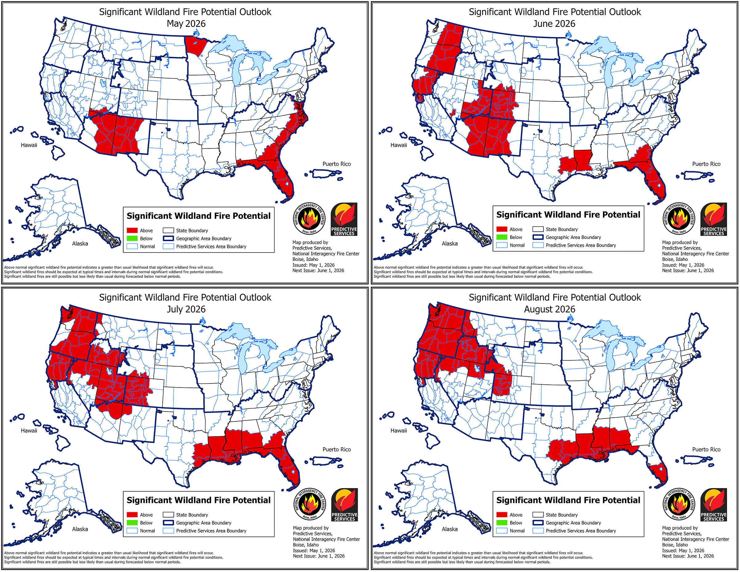
A warm, dry spring has set the stage for above-average significant wildland fire risk across much of the southern and western United States this summer, and no part of the United States will have below-average fire potential through the end of August.

These predictions are part of a 4-month outlook produced monthly by the National Interagency Fire Center (NIFC), a group of wildland fire experts from eight federal agencies that coordinates wildland fire resources across the country.

The most recent outlook, published 1 May, projects the likelihood of significant fires (defined as those that require an NIFC response) from May to August using long-term forecasts from NOAA’s Climate Prediction Center, current precipitation and drought conditions, and an assessment of the fuels available in different regions (like grasses, brush, and timber).

This year, 1,848,210 acres across the country have already burned—nearly twice the annual average over the past 10 years.

“It’s not necessarily a foregone conclusion that we’re going to have a really busy season, but everything is pointing that way,” said Jim Wallmann, a meteorologist for the U.S. Forest Service at the NIFC and one of the outlook’s authors.

Drought in the West

In the West, wildfire season typically peaks in late summer. This most recent outlook predicts an above-average significant fire potential for much of the West as the season peaks.

In May, the above-average risk is concentrated in eastern Arizona and western New Mexico, though that risk fades to normal by August as the Southwest’s monsoon season begins. In June, the above-average risk extends to western Colorado and parts of the Pacific Northwest. In July and August, that risk covers much of the Northwest, including Utah, Idaho, Oregon, Washington, and Northern California.

Above-average spring temperatures and a far-below-normal snowpack across the West are contributing to the elevated risk in Washington, Oregon, Idaho, and Northern California, in particular. Many river basins across the West contain less than 20% of their normal amount of snow, and some are already snow-free at all observed locations due to melting caused by warm temperatures in March.

“The snowpack being lower this time of year, and melting out, affects the soil moisture throughout the rest of the summer, which then affects the fuel moistures,” said Craig Clements, a meteorologist at San Jose State University’s Fire Weather Research Laboratory who was not involved in the outlook. Early snowmelt also uncovers fuels, like pine needles and leaf litter, that would typically be under snow, exposing them to the air to dry and catch fire.

Southern California and the Sierra Nevada mountain range, though, remain at an average significant fire risk throughout the summer, as a result of higher-than-average precipitation earlier in the year.

The Southeast and Beyond

Fire risk will also be elevated in the Southeast this summer. Florida, for example, remains at an above-average significant fire potential through the end of August. Southern Georgia, Mississippi, Louisiana, Arkansas, and the eastern halves of Virginia, North Carolina, and South Carolina will also have above-average significant fire potential.

The above-average risk is fueled, in part, by a worsening drought affecting the Southeast alongside the drought in the West. As of 1 May, nearly 63% of the country was experiencing drought, and 19% of the country was experiencing extreme or exceptional drought, according to the U.S. Drought Monitor.

The Midwest and the Northeast will remain at an average significant fire potential from May to August, though northwestern Minnesota faces an above-average potential in May.

No place in the United States is projected to have a below-average significant fire potential through the end of August.

Preparing Amid Uncertainty

A developing El Niño—a climate phenomenon that affects heat storage in the ocean—could alter the fire risk projections. Scientists expect that a strong El Niño could lead to a below-normal hurricane season, worsening drought in the Southeast. In the Pacific, a strong El Niño could intensify the hurricane season, which may lower wildfire risk.

However, a stronger El Niño could drive more lightning strikes in the Sierra Nevada, which could increase fire risk there, Clements said. In 2020, for example—a strong El Niño year—Hurricane Elida in the Pacific contributed to a lightning outbreak that supercharged wildfires in the West.

“We’re still not sure exactly how [El Niño] is going to impact the season,” Wallmann said. As late summer approaches, meteorologists will better understand how El Niño will develop and affect wildfire risk.

Weather patterns can change, and day-to-day conditions still play a role in fire occurrence. “If the weather shifts, or we get a really big heat wave, it can modify [the forecast]. Or if it remains relatively moderate, that might lessen the fire danger,” Clements said. “We’ll just have to see how the weather plays out.”

Wallmann and Clements emphasized that those living in areas with elevated fire risk should be aware of their surroundings and think ahead about where they might go for safety should a wildfire occur. “Having that situational awareness ahead of time can help you make better decisions,” Wallmann said.

—Grace van Deelen (@gvd.bsky.social), Staff Writer

Citation: van Deelen, G. (2026), Most of the U.S. West will face above-normal wildfire risk this summer, Eos, 107, https://doi.org/10.1029/2026EO260145. Published on 11 May 2026.

Text © 2026. AGU. CC BY-NC-ND 3.0
Except where otherwise noted, images are subject to copyright. Any reuse without express permission from the copyright owner is prohibited.

Source: Geophysical Research Letters

As seismic waves travel through Earth, they gradually lose energy, a process called attenuation. That energy loss doesn’t happen uniformly—some features in the crust sap far more energy from seismic waves than others. Researchers can map underground features by watching where seismic waves lose more or less energy. The Southern Array for the Lithosphere and Uplift of Taiwan Experiment (SALUTE) is doing just that, providing information that could lead to improved seismic hazard planning in the country.

Lin et al. report attenuation results from SALUTE focused on the convergence between the Eurasian plate and the Luzon Arc, an understudied, geologically dynamic area where Earth’s crust is deforming. Using the overall attenuation rate and relative attenuation rates of P and S seismic waves, the authors imaged active faults, identified distinct lithologies, and better resolved the Luzon forearc block that sits just offshore of Taiwan.

The authors used data from the SALUTE high-density seismographic network, spanning December 2020 to December 2023, to construct both 2D and 3D attenuation models. They found clear changes in attenuation associated with major faults, as well as areas of high attenuation associated with fluid-rich, ductile zones in the lower crust that cause tectonic tremors. Their attenuation imaging additionally revealed that the Luzon forearc block, which had been poorly imaged in the past, dips northward and narrows as it nears the convergence zone.

The authors say their results agree well with previous velocity-based seismic imaging studies and show that attenuation can image features, such as transition zones, that were previously difficult to capture. Their data could also be useful for better understanding seismic hazard throughout the region, they note. (Geophysical Research Letters, https://doi.org/10.1029/2025GL121583, 2026)

—Nathaniel Scharping (@nathanielscharp), Science Writer

Citation: Scharping, N. (2026), Seismic attenuation techniques reveal what lies beneath Taiwan, Eos, 107, https://doi.org/10.1029/2026EO260150. Published on 11 May 2026.

Text © 2026. AGU. CC BY-NC-ND 3.0
Except where otherwise noted, images are subject to copyright. Any reuse without express permission from the copyright owner is prohibited.

Thirty years ago, the blockbuster movie Twister featured a group of academics putting themselves at risk by chasing tornadoes in the name of science. Although the Hollywood story entailed a surfeit of sensationalism, special effects, and unrealistic stereotypes, the movie got a few things right. Specifically, the scientists were trying to study tornadoes using a large number of spatially distributed, home-built, low-cost (and potentially sacrificial) sensors.

Today, we commonly refer to the coordinated use of tens to hundreds of similar sensors that are spread out as “large-N” sensing. Such sensor distributions have led to important advances in seismology and infrasound science, where they have improved our understanding of seismic ground motion and helped shed light on volcanic eruption dynamics [e.g., Rosenblatt et al., 2022; Anderson et al., 2023].

The benefits of large-N networks and arrays include robust spatial sampling and signal extraction from noise. They are also advantageous for detecting small signals, sensing natural hazards in remote environments, and offering critical redundancies for sensors at risk from lava or debris flows, wildfire, weather, or even malicious mammals.

Since 2013, our research group in the Department of Geosciences at Boise State University (BSU) has worked to study infrasound from geophysical phenomena by capitalizing on the benefits of low-cost, large-N sensing technology [e.g., Slad and Merchant, 2021]. More than a decade on, this effort has yielded scientific successes from a variety of environments, and it is continuing to evolve.

Large-N Sensing for Infrasound

Many violent natural processes, including landslides, volcanic eruptions, earthquakes, avalanches, and meteors, produce infrasound, defined as low-frequency sound below the threshold of human hearing (less than 20 Hertz). Such events may create audible sound as well, but the subaudible band is often much more energetic in terms of sound intensity, and it has long wavelengths that can propagate long distances with little attenuation. These characteristics make infrasound especially valuable for remote sensing of natural phenomena.

Our group at BSU grew more interested in developing our own inexpensive infrasound sensing solutions after costing out technology for commercial data logging systems, the compact electronic devices that record and store sensor data. These systems can be far more expensive than infrasound transducers—the sensors that actually detect sound—themselves.

The cost element became particularly relevant after we lost instrumentation deployed at the summit of Chile’s Villarrica volcano when it erupted a 2-kilometer-tall lava fountain on 3 March 2015 [Johnson et al., 2018]. In an instant, our hardware, including seismic and infrasonic sensors and their commercial multichannel data loggers, was entombed beneath falling lava. This financial loss incentivized our work to develop low-cost loggers that would match the technical specifications and fidelity of commercial systems.

The result was the customized Gem infrasound logger, which we created using the widely available and very economical Arduino open-source electronic prototyping platform and its low–power consumption microcontroller. The Gem is an all-in-one infrasound sensor and data logger with a high dynamic range (millipascals to 100 pascals), a 100-hertz sample rate appropriate for infrasound, and a built-in GPS for precise timing and synchronization [Anderson et al., 2018].

Although we initially conceived of the Gem as an alternative to commercial loggers to be deployed as single stations or in small arrays, we quickly realized its potential for use in high-density distributed sensing arrays that enabled new detection capabilities. In particular, its small package size (it has about the dimensions and weight of a paperback novel) and its ease of deployment—simply insert alkaline batteries, place it on the ground, and turn it on—have opened opportunities for rapid, large-N deployments in difficult-to-access environments.

Early Successes for the Gem

The Gem’s inaugural field mission came in January 2020 during a return to Villarrica, where activity had returned to normal following its 2015 paroxysmal eruption [Rosenblatt et al., 2022]. Typical activity in the volcano’s normal state includes open-vent degassing from a small lava lake recessed deep within the summit crater, which produces its famously powerful volcano infrasound [e.g., Johnson et al., 2012].

To capture Villarrica’s infrasound in detail, a four-person team from BSU climbed the 3,000-meter-tall glaciated volcano and quickly installed 16 sensors around the crater rim, as well as another 16 sensors along an 8-kilometer linear transect from the summit down the northern slope (Figure 1). This unique sensor distribution permitted us to capture the infrasound wavefield and how it interacts with topography in unprecedented detail.

Deploying such an array configuration using much heavier, larger, and power-intensive conventional instruments would have taken far more time and resources, as well as a bigger group. With the Gems, however, the installation was feasible for our small team, each member of which could easily carry eight instruments and the batteries needed to power them.

Once in place, these sensors collected continuous data during the 2-week study that were used to quantify the diffraction of sound coming out of the volcanic crater [Rosenblatt et al., 2022] and to measure the sound’s attenuation as it propagated away. Such studies are important for investigating time-varying atmospheric parameters such as changing temperatures and winds, which can affect infrasound transmission, diminishing its amplitude or even—in extreme cases—completely silencing it in an acoustic shadow zone [Johnson et al., 2012]. To monitor volcanoes with infrasound, it is necessary to understand the influence of atmospheric effects.

Months later, another opportunity arose to demonstrate the Gems’ capability for large-N infrasound sensing. During the early days of the COVID-19 pandemic, on 31 March 2020, a magnitude 6.5 earthquake occurred near Stanley, Idaho. The earthquake, the largest in the state since 1983, kicked off an energetic aftershock sequence, with more than 700 magnitude 3 or greater earthquakes occurring in 6 months. Most of these events produced significant local infrasound radiation, or “airquakes,” caused by ground-atmosphere coupling [e.g., Johnson et al., 2020].

Pandemic-related precautions inhibited a large team from venturing as a group into the field. However, a lone BSU researcher (coauthor Jacob Anderson), trudging through forest terrain and deep snow on skis, was able to deploy and activate 22 Gems in less than 4 hours in early April, thanks in part to the sensors’ compact size and ease of deployment.

This array captured hundreds of local infrasonic aftershocks within about 25 kilometers of their epicenters. It also recorded a far larger event 700 kilometers away, the 15 May magnitude 6.5 Monte Cristo earthquake in Nevada. The array detected the epicentral infrasound from the distant earthquake source, as well as infrasound from numerous secondary sources, including mountain ranges throughout the western United States that reradiated the ground motion as infrasound (Figure 2) [Anderson et al., 2023].

Detecting all these distinct signals was possible because of the enhanced array processing capabilities provided by the large number of sensors. Anderson et al. [2023] showed that when the data were processed from 3-sensor subsets of the 20+-sensor array—instead of from the whole array—it was possible to detect only the most intense earthquake infrasound arrivals. In other words, the larger array had much greater fidelity and sensing capabilities than smaller distributions of sensors.

During its 2-month deployment, the Stanley array also detected sounds from other distant nonearthquake sources, including waterfalls 195 kilometers away and thunder more than 900 kilometers away [Scamfer and Anderson, 2023]. Such enhanced detections, facilitated by large-N sensing, demonstrate an improved capacity to monitor a range of Earth phenomena continuously over a wide range of distances.

Putting Sensors in Harm’s Way

Since those proof-of-concept deployments, Gems have been used to monitor snow avalanches, lahars, river flow discharge, stratospheric sounds (while mounted aboard a solar balloon), and numerous volcanoes during field experiments [e.g., Tatum et al., 2023; Bosa et al., 2024; Rosenblatt et al., 2022; Brissaud et al., 2021]. Given their ease of use, small size, and low replacement cost, they’ve also been tested in hazardous environments where the risk to more expensive hardware could be considered unreasonable.

The motivation to put sensors in harm’s way is to gain insight into geophysical phenomena by recording subtle signals close to the source that may not be detectable from farther away. For example, at Villarrica, Rosenblatt et al. [2022] suspended a Gem on a cable 100 meters above a lava lake to collect infrasound data from a unique, bird’s-eye perspective over the crater (Figure 1c). (Stringing the cable across the crater proved far more challenging than deploying the sensor itself, which slid down the cable until finding its resting place at the bottom of the cable’s arc.)

In another case, we landed a pair of Gems on the ground near a frequently exploding crater at Fuego volcano in Guatemala using a drone (see video below). We later retrieved one of the sensors from high on the volcano’s flanks. Another was lost because high winds initially posed too great a risk to fly the drone back for it. Then the following day after the wind subsided, we could not locate the stranded Gem, which was probably a casualty of a nighttime explosion.

Our group at BSU also has nascent interest in using Gems to study fire in natural environments. Wildfires produce infrasound from a spatially extensive source region corresponding to actively burning areas. Because of the source complexity and the fact that fire infrasound is low amplitude and tremor-like [Johnson et al., 2025], enhancing signal-to-noise ratios in recorded infrasound is critical. This enhancement is enabled by using large-N monitoring networks, making infrasound wildfire surveillance a promising area of investigation.

Toward this objective, our group installed 76 sensors ahead of a prescribed burn in Reynolds Creek, Idaho, in October 2023 to begin developing infrasound as a tool for monitoring and mapping wildfire. We have also deployed Gems for infrasound studies of naturally occurring wildfires, such as the Emigrant wildfire in Oregon in August and September 2025 (Figure 3). During that active wildfire response, a team safely and quickly installed tens of sensors within a matter of hours in an area facing dynamic hazards from the rapidly expanding fire, which eventually covered 33,000 acres (about 13,354 hectares). Luckily, no instruments were lost, and the data have shown the potential to track a wildfire as it advances.

Preliminary results suggest that low-cost, rapid infrasound deployments could one day be used as an effective operational tool. For example, in firefighting responses, infrasound might complement intermittent aerial observations, from aircraft or drones, because it provides a continuous record of fire activity. Infrasound surveillance might also be able to “hear” combustion sources within a burn area that is obscured to optical sensing because of clouds or nightfall.

The Evolution of Low-Cost Sensors

Five years ago, the single-sensor Gem was a cutting-edge infrasound logging solution. While it remains a powerful and economical tool for large-N arrays and for sensing in hostile environments, it is evolving.

We have now developed the Gem into an even more versatile version called the Aspen, which can log four independent sensors at a sample rate of 200 hertz, double that of the Gem. The Aspen retains the small size, low weight, low power consumption, and low cost of the Gem, but with the capability to record higher-resolution 24-bit, time-synchronized data from a triaxial seismic sensor and an infrasound transducer.

Recording synchronous seismoinfrasonic data on the same logging platform offers the advantage of sensing both ground shaking and infrasonic oscillations. The ability to measure waves propagating in the ground and in the air simultaneously could facilitate work in the growing field of environmental seismology, which focuses on geophysical sources at Earth’s surface like debris flows and volcanoes.

Although we have focused on seismoacoustic geophysical measurements in our work, the concept of gathering data with low-cost instrumentation in harm’s way or from coordinated arrays of numerous sensors holds promise across Earth and environmental sciences. Such approaches could be used, for example, with tiltmeters (which measure slope changes), gravity meters, or near-infrared thermometers (e.g., optical pyrometers), all of which would offer additional data streams complementing seismoacoustic observations in geophysical studies of volcanoes.

With the diversity of emerging uses, it’s clear that large-N sensing—infeasible or cost prohibitive in many cases until recently—could transform how we measure many facets of Earth, helping to reveal the inner workings of volatile volcanoes, twisting tornadoes, and more.

Acknowledgments

More information about low-cost infrasound sensing solutions can be found at https://sites.google.com/boisestate.edu/infravolc/home. Development of the Gem infrasound logging platform was supported by a grant from the National Science Foundation (EAR-2122188).

References

Anderson, J. F., et al. (2018), The Gem infrasound logger and custom‐built instrumentation, Seismol. Res. Lett., 89(1), 153–164, https://doi.org/10.1785/0220170067.

Anderson, J. F., et al. (2023), Remotely imaging seismic ground shaking via large-N infrasound beamforming, Commun. Earth Environ., 4(1), 399, https://doi.org/10.1038/s43247-023-01058-z.

Bosa, A. R., et al. (2024), Dynamics of rain-triggered lahars and destructive power inferred from seismo-acoustic arrays and time-lapse camera correlation at Volcán de Fuego, Guatemala, Nat. Hazards, 121, 3,431–3,472, https://doi.org/10.1007/s11069-024-06926-1.

Brissaud, Q., et al. (2021), The first detection of an earthquake from a balloon using its acoustic signature, Geophys. Res. Lett., 48, e2021GL093013, https://doi.org/10.1029/2021GL093013.

Johnson, J. B., et al. (2012), Probing local wind and temperature structure using infrasound from Volcan Villarrica (Chile), J. Geophys. Res., 117, D17107, https://doi.org/10.1029/2012JD017694.

Johnson, J. B., et al. (2018), Forecasting the eruption of an open-vent volcano using resonant infrasound tones, Geophys. Res. Lett., 45, 2,213–2,220, https://doi.org/10.1002/2017GL076506.

Johnson, J. B., et al. (2020), Mapping the sources of proximal earthquake infrasound, Geophys. Res. Lett., 47, e2020GL091421 , https://doi.org/10.1029/2020GL091421.

Johnson, J. B., J. F. Anderson, and K. Yedinak (2025), Infrasound produced by a small pile fire, Appl. Acoust., 231, 110559, https://doi.org/10.1016/j.apacoust.2025.110559.

Rosenblatt, B. B., et al. (2022), Controls on the frequency content of near-source infrasound at open-vent volcanoes: A case study from Volcán Villarrica, Chile, Bull. Volcanol., 84(12), 103, https://doi.org/10.1007/s00445-022-01607-y.

Scamfer, L. T., and J. F. Anderson (2023), Exploring background noise with a large‐N infrasound array: Waterfalls, thunderstorms, and earthquakes, Geophys. Res. Lett., 50, e2023GL104635, https://doi.org/10.1029/2023GL104635.

Slad, G., and B. Merchant (2021), Evaluation of Low Cost Infrasound Sensor Packages, Sandia Rep. SAND2021-13632, Sandia Natl. Lab., Albuquerque, N.M., https://doi.org/10.2172/1829264.

Tatum, T., J. F. Anderson, and T. J. Ronan (2023), Whitewater sound dependence on discharge and wave configuration at an adjustable wave feature, Water Resour. Res., 59, e2023WR034554, https://doi.org/10.1029/2023WR034554.

Author Information

Jeffrey B. Johnson (jeffreybjohnson@boisestate.edu), Jacob F. Anderson, Madeline A. Hunt, Owen A. Walsh, and Jerry C. Mock, Department of Geosciences, Boise State University, Idaho

Citation: Johnson, J. B., J. F. Anderson, M. A. Hunt, O. A. Walsh, and J. C. Mock (2026), Sensing the sounds from Earth’s hazardous environments, Eos, 107, https://doi.org/10.1029/2026EO260142. Published on 8 May 2026.

Text © 2026. The authors. CC BY-NC-ND 3.0
Except where otherwise noted, images are subject to copyright. Any reuse without express permission from the copyright owner is prohibited.

Emissions from urban areas account for about a tenth of the global methane budget, according to a new analysis of satellite data published in the Proceedings of the National Academy of Sciences of the United States of America. And those emissions grew by about 10% from 2020 to 2023, despite cities’ pledges to slash them.

Methane is a potent greenhouse gas, and it’s shorter lived in the atmosphere than carbon dioxide. That means cutting methane emissions would have great benefits for the climate over the short term. Oil and gas operations and agriculture are major sources of methane, but so are cities and their infrastructure.

“Cities have started attempting to reduce their methane emissions, and we hope to be able to monitor this,” said Erica Whiting, a graduate student in climate and space science at the University of Michigan. Most efforts to account for urban methane emissions—from wastewater treatment plants, landfills, leaky natural gas infrastructure, and other sources—have relied on ground-based measurements and on inventories that estimate emissions on the basis of activities, said Whiting. Most of these studies have looked at a handful of cities, typically in North America and Europe.

In contrast, Whiting said her team’s study is one of the first to use satellite data to monitor urban methane emissions over time. Satellite monitoring offers long-term, often global, measurements and can provide a clearer picture of how mitigation efforts are developing.

Falling Short

A growing number of cities are aiming to reduce carbon emissions, and the new data show many of them are not on track. Whiting’s study included 92 cities around the world, including 51 members of a coalition called C40, which was founded in 2005. This 96-country coalition is working toward the goal of cutting greenhouse gas emissions by half by 2030, including a 34% decrease in methane emissions. These numbers are aligned with the goal of limiting global warming to 1.5°C over preindustrial levels.

Whiting’s team analyzed methane data from the satellite-based TROPOMI (Tropospheric Monitoring Instrument) from 2019 to 2023. TROPOMI launched in 2017, making it possible to continuously monitor methane and other gas concentrations around the world. TROPOMI data showed that from 2019 to 2020, urban methane levels fell. But from 2020 to 2023, emissions grew 10% in C40 cities and 12% in non-C40 cities. The study focuses not just on urban centers but also on their outlying areas, where known methane sources such as landfills and wastewater treatment plants are often located.

The current study can’t point to what accounts for these trends, said Whiting. However, she said, urban populations grew during the study period, which could be a contributor to the cities’ growing emissions.

Rob Jackson, an Earth system scientist at Stanford University and chair of the Global Carbon Project, noted that it’s hard to know how to interpret the increase in emissions because the study period includes the era of the COVID-19 pandemic lockdowns, which caused major changes in people’s behavior and associated drops in anthropogenic emissions in 2020. (However, counterintuitively, the early 2020s actually saw a spike in overall methane emissions, which some scientists attribute to wetlands and changes in atmospheric chemistry.) Nevertheless, he said the data show that the world is not on track to decrease urban methane emissions. “In most regions of the world, there is no evidence that methane emissions from cities are decreasing at all,” he said.

“This work clearly shows that major cities worldwide are not reducing methane emissions at a rate consistent with the Global Methane Pledge,” Jackson said. This international agreement, made in 2021, has reduction goals that align with those of the C40 coalition: decrease global methane emissions by at least 30% relative to 2020 levels by 2030. The European Commission and 159 countries are participating in the pledge.

Whiting hopes better data will help. City and regional governments can use data from satellites to support and monitor ongoing efforts to lower methane emissions. “We’re excited to have this approach to monitor changes, and it should be useful for urban planning,” she said.

Zachary Tofias, director of food and waste at C40 Cities, noted via email that the organization was not involved with the design of the study. He pointed to several recent large-scale composting and other waste management facilities recently commissioned by member cities that should help bring down methane emissions going forward. The increasing availability of satellite and aerial monitoring data, he said, “provides an amazing additional tool for cities and facility managers to understand and address methane leaks from waste-disposal sites.”

—Katherine Bourzac (@bourzac.bsky.social), Science Writer

Citation: Bourzac, K. (2026), Urban methane emissions are rising, despite cities’ pledges, Eos, 107, https://doi.org/10.1029/2026EO260143. Published on 8 May 2026.

Text © 2026. The authors. CC BY-NC-ND 3.0
Except where otherwise noted, images are subject to copyright. Any reuse without express permission from the copyright owner is prohibited.