Editors’ Highlights are summaries of recent papers by AGU’s journal editors.
Source: AGU Advances
The evolution of rivers that split into multiple channels is a scientific challenge in terms of modeling and prediction. On the other hand, these rivers are widespread and play a key role for ecosystems’ life, groundwater recharge, and therefore, water security. They are also extremely sensitive to hydroclimatic changes, leading to shifts in precipitation, erosion and sediment transport.
Z
The evolution of rivers that split into multiple channels is a scientific challenge in terms of modeling and prediction. On the other hand, these rivers are widespread and play a key role for ecosystems’ life, groundwater recharge, and therefore, water security. They are also extremely sensitive to hydroclimatic changes, leading to shifts in precipitation, erosion and sediment transport.
Zhao et al. [2026] investigate the drivers of river evolution for 97 multithread river reaches worldwide, spanning diverse climates and morphologies. The study reveals the key role of intermittency for river evolution. In particular, higher flow intermittency could lead to more even flow partitioning among threads, therefore impacting hydrology and ecosystems. With flow variability increasing after climate change, rivers are likely to increase their thread count, thus impacting livelihoods and ecosystems.
Two example multithread reaches shown in Landsat images from (b) the Irtysh River (wandering) and (c) the Yukon River (braided). Credit: Zhao et al. [2026], Figure 1(b,c)
Citation: Zhao, F., Ganti, V., Chadwick, A., Greenberg, E., McLeod, J., Liu, Y., et al. (2026). Global hydroclimatic controls on multithread River dynamics. AGU Advances, 7, e2025AV002166. https://doi.org/10.1029/2025AV002166
As the Indian and Eurasian continental plates collide, the Tibetan Plateau is slowly deforming. For decades, geoscientists debated how this deformation occurs: Is the plateau like a block of crumbly aged cheddar, deforming mostly at its faults, or is it more like French brie, moving like a very viscous liquid being pushed slowly to the east?
A new study published in Science shows that both theories are at work. The study’s findings provide the most comprehensive picture yet of the Tibetan Pl
As the Indian and Eurasian continental plates collide, the Tibetan Plateau is slowly deforming. For decades, geoscientists debated how this deformation occurs: Is the plateau like a block of crumbly aged cheddar, deforming mostly at its faults, or is it more like French brie, moving like a very viscous liquid being pushed slowly to the east?
A new study published in Science shows that both theories are at work. The study’s findings provide the most comprehensive picture yet of the Tibetan Plateau’s deformation and offer valuable information for earthquake hazard assessments in the region.
The new model that combines the two theories is a “significant advance,” said Eric Fielding, a geodesist who was not involved in the study. Fielding is a staff member at NASA’s Jet Propulsion Laboratory but did not speak on behalf of the agency. “It’s clearly the result of a very large amount of work,” he said.
A Deformation Investigation
For decades, scientists have held differing views on the Tibetan Plateau’s deformation. One camp modeled the plateau’s deformation with movement occurring mostly at its faults, while the other modeled the movement like a thick fluid deforming areas beyond faults.
“These two communities have carried on modeling deformation in different ways” and have never fully resolved the differences between their models, said Tim Wright, a geodesist at the University of Leeds in the United Kingdom and lead author of the new study.
It’s tricky to measure the plateau’s deformation, though, because it changes so slowly: One of the fastest faults on the plateau, the Kunlun Fault, moves at about just 10 millimeters per year. “These are rates that are less than your fingernails growing,” Wright said.
And because much of the Tibetan Plateau’s terrain is inaccessible, there’s a dearth of ground-based stations to track movement, meaning most geodetic data for the area must come from satellites.
“It’s a boon for science to have that consistent acquisition of the same kind of data for 10 years.”
Tracking such nearly imperceptible movement with satellites hundreds of kilometers above requires enormous amounts of data collected over many years. Wright and his colleagues finally had those data after 10 years of observations from the European Space Agency’s Sentinel-1 satellite mission, which launched in 2014.
“Because the signals are so small, you need to wait for some time before you accrue enough deformation that you can actually measure it,” Wright said. The 2014–2024 data they analyzed are “giving us a really clean signal,” he said.
“It’s a boon for science to have that consistent acquisition of the same kind of data for 10 years,” Fielding said.
Using tens of thousands of satellite images alongside ground-based satellite navigation system stations, Wright and the team constructed comprehensive velocity maps of the deformation of the plateau. Results showed that a mix of theories best describes the mechanism.
“We think what’s really happening is a combination of both,” Wright said.
Wright, who described himself as “formerly of the viscous deformation camp,” was surprised by the prominent role that faults played in the plateau’s deformation. Previously, he said, he would have described the faults as passive markers within the underlying flow of the landmass. But the data show that the faults influence a much broader area of the plateau: “The whole deformation of the plateau is influenced by those faults,” he said.
The study “shows clearly that these major fault systems are responsible for a large part of the strain within the plateau,” Fielding said.
Mapping Seismic Hazards
“We have very little information about the history of earthquakes on these faults in this area.”
Knowing how the plateau deforms can also help scientists create more accurate seismic hazard assessments for the millions of people who may be affected by earthquakes there, particularly at the edges of the plateau. “We have very little information about the history of earthquakes on these faults in this area,” Fielding said.
The research team is working with the Global Earthquake Model Foundation, a nonprofit earthquake research collaboration, and other organizations to incorporate their findings into hazard assessments.
Wright and the research team recently used a similar methodology to map the deformation field of the entire Alpine-Himalayan belt, which stretches from Spain to eastern China. The same methods could be used to map the deformation of the western United States, another area where both viscous and fault-related deformation may affect large population centers, Fielding said.
Citation: van Deelen, G. (2026), Weak faults play a strong role in the Tibetan Plateau’s deformation, Eos, 107, https://doi.org/10.1029/2026EO260162. Published on 22 May 2026.
About two tons of satellite material burns up in Earth’s atmosphere every day. That is the steady-state exhaust of a single company’s broadband network, SpaceX’s Starlink, operating at its current scale. Each vaporized spacecraft leaves behind aluminum oxide, lithium, copper, and a growing list of metals the upper atmosphere has never had to contained in these quantities before.
We’re following a familiar human pattern. A commons, like the low earth orbit (LEO) region of space, is declared abund
About two tons of satellite material burns up in Earth’s atmosphere every day. That is the steady-state exhaust of a single company’s broadband network, SpaceX’s Starlink, operating at its current scale. Each vaporized spacecraft leaves behind aluminum oxide, lithium, copper, and a growing list of metals the upper atmosphere has never had to contained in these quantities before.
We’re following a familiar human pattern. A commons, like the low earth orbit (LEO) region of space, is declared abundant. Commercial activity scales faster than science can measure the consequences. Governance lags by a decade or more. By the time the damage is legible, it is already expensive to reverse.
We did this to rivers in the 19th century, to the atmosphere in the 20th, and to the deep ocean in a quiet accumulation that stretched across both. A new peer-reviewed analysis published in Advances in Space Research makes clear that LEO is now on the same trajectory, and the chemistry is moving faster than the regulation.
An Atmosphere Already Dominated by Human Metal
The paper, an update to a 2021 study, reassesses how much spacecraft material is now being injected into the mesosphere and lower thermosphere as satellites and rocket stages burn up on reentry. The comparison it draws is that for several metals commonly used in spacecraft, anthropogenic injection now rivals or exceeds the natural input from meteoroids.
What was already true in 2021 is more true now. The researchers incorporate direct observations from stratospheric aerosol sampling — work led by Daniel Murphy at NOAA and published in PNAS in 2023 — which confirmed that roughly 10 percent of stratospheric aerosol particles now contain aluminum and other metals traceable to satellite and rocket-stage burn-up. For decades, the natural baseline was micrometeoroid ablation, what space sent naturally toward our planet. Earth sweeps up roughly 30 to 50 metric tons of cosmic dust every day, a steady rain of mostly sand-grain-sized particles left over from comets and asteroids. Those grains hit the upper atmosphere at speeds between 11 and 72 kilometers per second, vaporize in a thin layer between about 75 and 110 kilometers altitude, and seed the mesosphere with iron, magnesium, silicon, sodium, and trace amounts of nickel, calcium, and aluminum. This process has been running for the entire 4.5-billion-year history of the planet. The metal layers it produces in the upper atmosphere are well-mapped; they are the chemistry the stratosphere evolved with.
Aluminum is a useful tracer because it is a small share of the natural input. Cosmic dust is dominated by silicates and iron, with aluminum running on the order of one to two percent by mass. So when researchers began detecting elevated aluminum in stratospheric aerosol particles in the early 2020s, the signal was unambiguous — meteoritic infall could not account for it. The source had to be terrestrial in origin, vaporized at altitude. Spacecraft, in other words.
Human vehicles have become a second, larger source.
The near-term trajectory is worse. Researchers at the University of Southern California documented an eightfold increase in stratospheric aluminum oxide between 2016 and 2022, corresponding almost exactly to the ramp-up of Starlink and other satellite megaconstellations. In 2022 alone, reentering satellites released an estimated 17 metric tons of aluminum oxide nanoparticles — raising total atmospheric aluminum input about 29.5 percent above natural levels.
The Ocean Parallel
Consider the deep ocean in the 1960s. Dumping was legal, monitoring was barely funded, and the prevailing assumption was that the ocean was big enough to absorb anything. We now know the answer to that assumption after finding microplastics in Mariana Trench amphipods, pharmaceutical residues in Arctic sediment cores, and PFAS in polar bear blood.
Low Earth orbit is in the 1960s-ocean phase. The prevailing assumption among launch operators is that satellites that burn up are satellites that disappear. Michael Byers, Canada Research Chair in global politics and international law, put this directly in a 2024 interview with Scientific American: “There’s this widespread assumption that something burning up in the atmosphere disappears, but, of course, mass never disappears.”
What it does instead is change form. A 250-kilogram satellite, typically about 30 percent aluminum by mass, generates roughly 30 kilograms of aluminum oxide nanoparticles as it ablates through the mesosphere. Those particles are small enough — 1 to 100 nanometers — that they can drift in the stratosphere for decades before settling. Aluminum oxide is not inert. It catalyzes the chlorine reactions that destroy stratospheric ozone, the same chemistry the Montreal Protocol was designed to stop. Crucially, the particles are not consumed in those reactions; they continue to destroy ozone molecules for the duration of their atmospheric lifetime.
The Scale Is Not Hypothetical
As of April 2026, SpaceX alone operates more than 10,000 active Starlink satellites, roughly two-thirds of all functioning spacecraft in orbit. The company has launched over 11,700 total, with about 1,500 already deorbited and replaced. Starlink satellites are designed for a five-year operational life, which means the constellation is, by design, a continuous churn: launch, operate, burn, launch again.
Amazon’s Project Kuiper, Eutelsat’s OneWeb, and a growing roster of Chinese state-backed constellations are moving toward similar architectures. The European Space Agency now tracks roughly 40,000 objects in low Earth orbit, about 11,000 of them active payloads, the rest debris or derelict hardware. Statistical models from ESA estimate another 130 million fragments smaller than one centimeter, each traveling fast enough to destroy whatever it hits.
Research published in Geophysical Research Letters projects that once currently planned megaconstellations are fully deployed, roughly 912 metric tons of aluminum will reenter the atmosphere every year, producing around 360 tons of aluminum oxide annually. A separate NOAA modeling study published in 2025 found that sustained alumina injection at expected 2040 levels could alter polar vortex speeds, warm parts of the mesosphere by as much as 1.5°C, and measurably impact the ozone layer.
Two Kinds of Pollution, One Commons
The orbital damage is happening on two fronts simultaneously, and they reinforce each other.
Atmospheric injection is the slow-accumulating chemistry problem. Every satellite that completes its mission becomes tomorrow’s stratospheric dust. A newly upgraded lidar system at the Leibniz Institute of Atmospheric Physics in Germany can now simultaneously detect lithium, sodium, copper, titanium, silicon, gold, silver, and lead in the upper atmosphere — each element a chemical fingerprint for specific spacecraft components. On February 20, 2025, the instrument registered a sudden spike in lithium vapor that researchers traced to a Falcon 9 upper stage reentering overhead.
The measurement capability is arriving just as the pollution is scaling.
Orbital debris is the faster-moving physical problem. SpaceX reported that its Starlink satellites executed 144,404 collision-avoidance maneuvers in the first half of 2025, due to collision warnings every couple of minutes, for six months straight — three times the previous rate. Two Starlink satellites have fragmented in orbit in the past four months, each creating a trackable debris field. Space is getting filled with junk that led to the International Space Station performing avoidance maneuvers twice in a single six-day window in November 2024, and again in April 2025.
Darren McKnight, a senior technical fellow at the debris-tracking firm LeoLabs, told IEEE Spectrum that certain orbital altitudes at 775, 840, and 975 kilometers have already passed the debris-density threshold where collisions generate fragments faster than atmospheric drag can remove them. This is known as the Kessler syndrome, proposed by NASA scientists Donald Kessler and Burton Cour-Palais in 1978, and it is no longer hypothetical in every band.
“Some operators in low Earth orbit are ignoring known long-term effects of behavior for short-term gain,” McKnight said, “Some will not change behavior until something bad happens.”
The Governance Gap
There is no body that regulates the cumulative atmospheric impact of satellite reentries. No operator is required to submit an environmental impact assessment for a constellation’s aggregate burn-up.
The FCC licenses spectrum.
National launch authorities license liftoff.
Debris mitigation guidelines from the UN’s Committee on the Peaceful Uses of Outer Space are voluntary, and compliance is inconsistent. The chemistry of the upper atmosphere is, in regulatory terms, nobody’s jurisdiction.
The United Nations Environment Program took a first step in late 2025, releasing a report titled Safeguarding Space: Environmental Issues, Risks and Responsibilities. It framed space debris and atmospheric injection as “emerging issues” deserving the attention international bodies already give to ocean pollution and transboundary air quality. This is the same framing UNEP used for atmospheric ozone depletion in the 1970s before the Montreal Protocol. Measuring something does not fix it. But it is the necessary precondition for fixing it — and for the first time, the measurement infrastructure is catching up to the pollution.
The Counter-Case, Honestly
Not every specialist agrees the situation is as urgent as the headlines suggest. A skeptical review published in March 2026 argued that the Kessler cascade framing oversimplifies a risk that plays out on timescales of decades to centuries, and in specific orbital bands rather than across all of LEO. The review is right on one narrow point: the ISS has operated continuously at 400 kilometers since 2000, its debris risk is managed in real time, and the environment is not in a runaway state.
What the skeptical case does not resolve is the atmospheric chemistry. The Kessler debate is about whether low-earth orbit becomes unusable. The alumina question is about whether the recovery of the ozone layer — a genuine success story of international environmental governance — is quietly being undone from above. Those are different problems. The first might take a century. The second is already measurable and is projected to worsen within fifteen years.
Emissions from urban areas account for about a tenth of the global methane budget, according to a new analysis of satellite data published in the Proceedings of the National Academy of Sciences of the United States of America. And those emissions grew by about 10% from 2020 to 2023, despite cities’ pledges to slash them.
Methane is a potent greenhouse gas, and it’s shorter lived in the atmosphere than carbon dioxide. That means cutting methane emissions would have great benefits for the clim
Emissions from urban areas account for about a tenth of the global methane budget, according to a new analysis of satellite data published in the Proceedings of the National Academy of Sciences of the United States of America. And those emissions grew by about 10% from 2020 to 2023, despite cities’ pledges to slash them.
Methane is a potent greenhouse gas, and it’s shorter lived in the atmosphere than carbon dioxide. That means cutting methane emissions would have great benefits for the climate over the short term. Oil and gas operations and agriculture are major sources of methane, but so are cities and their infrastructure.
“Cities have started attempting to reduce their methane emissions, and we hope to be able to monitor this,” said Erica Whiting, a graduate student in climate and space science at the University of Michigan. Most efforts to account for urban methane emissions—from wastewater treatment plants, landfills, leaky natural gas infrastructure, and other sources—have relied on ground-based measurements and on inventories that estimate emissions on the basis of activities, said Whiting. Most of these studies have looked at a handful of cities, typically in North America and Europe.
In contrast, Whiting said her team’s study is one of the first to use satellite data to monitor urban methane emissions over time. Satellite monitoring offers long-term, often global, measurements and can provide a clearer picture of how mitigation efforts are developing.
Falling Short
A growing number of cities are aiming to reduce carbon emissions, and the new data show many of them are not on track.
A growing number of cities are aiming to reduce carbon emissions, and the new data show many of them are not on track. Whiting’s study included 92 cities around the world, including 51 members of a coalition called C40, which was founded in 2005. This 96-country coalition is working toward the goal of cutting greenhouse gas emissions by half by 2030, including a 34% decrease in methane emissions. These numbers are aligned with the goal of limiting global warming to 1.5°C over preindustrial levels.
Whiting’s team analyzed methane data from the satellite-based TROPOMI (Tropospheric Monitoring Instrument) from 2019 to 2023. TROPOMI launched in 2017, making it possible to continuously monitor methane and other gas concentrations around the world. TROPOMI data showed that from 2019 to 2020, urban methane levels fell. But from 2020 to 2023, emissions grew 10% in C40 cities and 12% in non-C40 cities. The study focuses not just on urban centers but also on their outlying areas, where known methane sources such as landfills and wastewater treatment plants are often located.
The Tropospheric Monitoring Instrument (TROPOMI) aboard the Sentinel-5P satellite measures the potent greenhouse gas methane. In snapshots over urban areas, higher methane concentrations are depicted in warmer colors. Credit: Erica Whiting
The current study can’t point to what accounts for these trends, said Whiting. However, she said, urban populations grew during the study period, which could be a contributor to the cities’ growing emissions.
“In most regions of the world, there is no evidence that methane emissions from cities are decreasing at all.”
Rob Jackson, an Earth system scientist at Stanford University and chair of the Global Carbon Project, noted that it’s hard to know how to interpret the increase in emissions because the study period includes the era of the COVID-19 pandemic lockdowns, which caused major changes in people’s behavior and associated drops in anthropogenic emissions in 2020. (However, counterintuitively, the early 2020s actually saw a spike in overall methane emissions, which some scientists attribute to wetlands and changes in atmospheric chemistry.) Nevertheless, he said the data show that the world is not on track to decrease urban methane emissions. “In most regions of the world, there is no evidence that methane emissions from cities are decreasing at all,” he said.
“This work clearly shows that major cities worldwide are not reducing methane emissions at a rate consistent with the Global Methane Pledge,” Jackson said. This international agreement, made in 2021, has reduction goals that align with those of the C40 coalition: decrease global methane emissions by at least 30% relative to 2020 levels by 2030. The European Commission and 159 countries are participating in the pledge.
Whiting hopes better data will help. City and regional governments can use data from satellites to support and monitor ongoing efforts to lower methane emissions. “We’re excited to have this approach to monitor changes, and it should be useful for urban planning,” she said.
Zachary Tofias, director of food and waste at C40 Cities, noted via email that the organization was not involved with the design of the study. He pointed to several recent large-scale composting and other waste management facilities recently commissioned by member cities that should help bring down methane emissions going forward. The increasing availability of satellite and aerial monitoring data, he said, “provides an amazing additional tool for cities and facility managers to understand and address methane leaks from waste-disposal sites.”
Citation: Bourzac, K. (2026), Urban methane emissions are rising, despite cities’ pledges, Eos, 107, https://doi.org/10.1029/2026EO260143. Published on 8 May 2026.
When it comes to thriving at high elevation, diminutive plants are always a safe bet. And low-lying vegetation is in fact colonizing higher and higher reaches as the climate changes, new results reveal. Researchers analyzed more than 2 decades’ worth of satellite data and showed that the vegetation line in the Himalayas is moving upward, in some cases by up to several meters per year. These changes have implications for the hydrology of the region and therefore for water resources for the popul
When it comes to thriving at high elevation, diminutive plants are always a safe bet. And low-lying vegetation is in fact colonizing higher and higher reaches as the climate changes, new results reveal. Researchers analyzed more than 2 decades’ worth of satellite data and showed that the vegetation line in the Himalayas is moving upward, in some cases by up to several meters per year. These changes have implications for the hydrology of the region and therefore for water resources for the population centers located downstream, the team reported last month in Ecography.
Mountains and People
“If you’re going to understand climate change across the Himalayas, you can’t just look at one location.”
The Himalayas, with their massive stores of frozen water, are part of a region known as the planet’s “Third Pole.” Nearly a billion people rely on water sourced from this area, but the Himalayas aren’t immune to climate change—shifts in temperature and precipitation patterns are causing glaciers to melt and permafrost to thaw, among other effects. “The Himalayan mountains are experiencing a lot of ecosystem changes,” said Ruolin Leng, an Earth scientist who led this new research while at the University of Exeter in the United Kingdom. She currently works at H2Tab, a wellness company.
And while the macroscopic effects of climate change in mountainous regions—the melting of the aforementioned glaciers, for example—have been readily studied, shifts in vegetation are often overlooked, said Leng. That’s a problem because plant cover affects everything from soil moisture levels to water runoff to the albedo of the planet’s surface, all of which have consequences for how water moves through the larger system, she said. “It’s a very important factor in the hydrological system.”
Leng and her colleagues focused on six sites, each roughly 40,000 square kilometers in size, in Bhutan, Nepal, and politically disputed areas farther west. Altogether the locales spanned roughly 15° in longitude (about the width of a U.S. time zone). The choice to analyze several locations along an east-west gradient was deliberate, said Stephan Harrison, a climate scientist also at the University of Exeter and a member of the research team. “The western Himalayas are very different from the eastern Himalayas in terms of climate. If you’re going to understand climate change across the Himalayas, you can’t just look at one location.”
Spotting Vegetation from Space
For each of those sites, the researchers mined satellite observations collected from 1999 to 2022 by the NASA/U.S. Geological Survey Landsat program. The researchers focused on visible and near-infrared observations to calculate a metric known as the normalized difference vegetation index (NDVI). Vegetation tends to reflect relatively little visible light while reflecting much more near-infrared light, and that fact can be exploited to infer the presence of vegetation in remote sensing data, said Karen Anderson, a remote sensing scientist at the Environment and Sustainability Institute at the University of Exeter and a member of the research team.
After masking out pixels too obscured by clouds or snow to correctly analyze, Leng and her colleagues calculated the NDVI for each 30- × 30-meter Landsat pixel within their study regions. The team retained pixels with NDVI levels above a minimum threshold and used those data, combined with topography information, to estimate the maximum elevation that was reliably vegetated each year. All six sites exhibited upward trends in the elevations of their vegetation lines over time, the researchers found. A site in central Nepal straddling the country’s northern border recorded the largest changes: From 1999 to 2022, the elevation of its vegetation line rose from roughly 5,520 meters to 5,670 meters, an increase of just under 7 meters per year on average. The five remaining sites all recorded annual upward shifts ranging from about 1 to 6 meters per year on average.
“Broadly speaking, plants are moving up mountains,” said Anderson. But different regions are responding differently, she added. (And while similar results have been previously noted in the Himalayas, not all plant life everywhere is moving up—recent research has shown that some tree lines are in fact moving downslope.)
A Climatic Culprit?
“People neglect the little plants.”
To investigate the potential drivers behind these changes, the team studied correlations with three climatic parameters: temperature, total precipitation, and snow depth. These data came from the European Centre for Medium-Range Weather Forecasts reanalysis dataset, which has a spatial resolution of roughly 30 kilometers.
Leng and her collaborators found that their site with the fastest-changing vegetation line also recorded the most rapid increase in snow depth over time. These two changes might therefore be linked, but more work is needed, Anderson admitted. “We haven’t addressed the causal link here. We’ve simply looked for patterns.”
There’s also a significant mismatch in the spatial resolution of the team’s meteorological data and their Landsat data, said Trevor Keenan, an ecosystem scientist at the University of California, Berkeley not involved in the research. Such a discrepancy can be particularly problematic in complex landscapes like mountain ranges because the coarse meteorological data might not be capturing the true microclimates that are bound to persist in such places, he said. “With heterogenous terrain and large elevational gradients, you really need that microclimate information.”
Sagarmatha National Park in Nepal, home to Mount Everest, is also host to rhododendron forests like this one. Credit: Peter Prokosch, CC BY-NC-SA 2.0
Anderson knows the geographical complexity of the Himalayas firsthand—in 2017 and 2022, she and other scientists conducted fieldwork in Nepal that informed this research. Those trips were a special opportunity to see plants like dwarf rhododendron thriving in tough conditions, she said. And it was a good lesson in appreciating some of the most diminutive members of the plant kingdom, Anderson added. “People neglect the little plants.”
Editors’ Highlights are summaries of recent papers by AGU’s journal editors.
Source: AGU Advances
Aerosols are tiny particles suspended in the air. They can cool the climate by making clouds brighter and longer-lasting. Scientists rely on satellite observations to measure the aerosol-cloud interaction, but distinguishing human impacts from natural weather patterns remains a challenge.
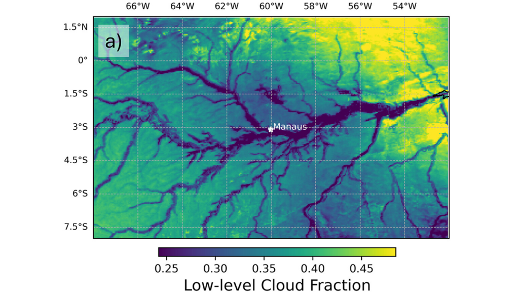
Christensen et al. [2026] reveal that the Amazon River itself creates cloud patterns that mimic the si
Aerosols are tiny particles suspended in the air. They can cool the climate by making clouds brighter and longer-lasting. Scientists rely on satellite observations to measure the aerosol-cloud interaction, but distinguishing human impacts from natural weather patterns remains a challenge.
Christensen et al. [2026] reveal that the Amazon River itself creates cloud patterns that mimic the signatures of pollution. Using 15 years of satellite data, researchers found that the temperature difference between the cool river and the warm land drives a local “river breeze” circulation. This natural process creates clouds with smaller and more numerous water droplets, which exhibit very similar features that satellites look for to identify pollution. Consequently, clean clouds over the river can appear polluted in satellite datasets. These findings highlight the critical need to account for local geography and natural weather patterns to accurately assess how human activities are influencing Earth’s climate.
Citation: Christensen, M. W., Varble, A. C., Tai, S.-L., Wind, G., Meyer, K., Holz, R., et al. (2026). The Amazon River-breeze circulation limits detection of aerosol-cloud interactions in warm clouds. AGU Advances, 7, e2025AV002188. https://doi.org/10.1029/2025AV002188
Editors’ Highlights are summaries of recent papers by AGU’s journal editors.
Source: AGU Advances
In low Earth orbit (typically below about 700 kilometers altitude), atmospheric drag is the primary source of uncertainty when predicting the trajectories of satellites. These prediction errors largely arise from limitations and inaccuracies in the models used to estimate the density of the upper atmosphere, particularly within the thermosphere.
Mutschler et al. [2026] introduce a new met
In low Earth orbit (typically below about 700 kilometers altitude), atmospheric drag is the primary source of uncertainty when predicting the trajectories of satellites. These prediction errors largely arise from limitations and inaccuracies in the models used to estimate the density of the upper atmosphere, particularly within the thermosphere.
Mutschler et al. [2026] introduce a new method for estimating atmospheric density along the path of an individual satellite by using Energy Dissipation Rates (EDRs). The derived single-satellite density measurements provide valuable insight into variations in thermospheric density and can help characterize how the upper atmosphere responds to disturbances such as geomagnetic storms. Incorporating these observations can contribute to ultimately improving the accuracy of satellite orbit predictions.
Effective density and Space Force effective density estimated by the Kosmos 1508 satellite (plotted on the right-hand y axes) compared to estimates from satellites Swarm-A and Swarm-C (plotted on the left-hand y-axes). Credit: Mutschler et al. [2026], Figure 17a
Citation: Mutschler, S., Pilinski, M., Zesta, E., Oliveira, D. M., Delano, K., Garcia-Sage, K., & Tobiska, W. K. (2026). First results of a new inversion tool for thermospheric neutral mass density computations during severe geomagnetic storms. AGU Advances, 7, e2025AV002079. https://doi.org/10.1029/2025AV002079
Editors’ Vox is a blog from AGU’s Publications Department.
As climate change increases the frequency and intensity of flooding, it’s becoming increasingly important to monitor and predict flood hazards at different scales. A new article in Reviews of Geophysics presents a data-driven performance analysis of various space-based sensors that monitor flood hazards. Here, we asked the lead author to give an overview of satellite-based flood monitoring, the benefits and challenges of using satell
As climate change increases the frequency and intensity of flooding, it’s becoming increasingly important to monitor and predict flood hazards at different scales. A new article in Reviews of Geophysics presents a data-driven performance analysis of various space-based sensors that monitor flood hazards. Here, we asked the lead author to give an overview of satellite-based flood monitoring, the benefits and challenges of using satellite-based sensors, and future space-based projects.
Why is it important to monitor the surface waters on Earth?
More than half of the world’s population lives within three kilometers of a freshwater body. When seasonal flooding behaves as anticipated, it provides essential nutrient replenishment to soils and crops. However, extreme flooding disturbs the careful balance of freshwater systems and can cause damaging flooding that disrupts livelihoods.
Climate change is making these extremes more frequent and less predictable, while expanding populations in flood-prone areas amplify the human cost. Continuous monitoring of Earth’s surface waters is essential as it helps us anticipate hazards, evaluate risk, and design interventions that protect the people and places most exposed to hydrologic hazards.
What are the benefits of monitoring flood inundation from space compared to other techniques?
Monitoring flood inundation from space is advantageous due to the wide-scale global coverage that captures important information over large areas. In-situ sensors, such as river gauges, provide valuable data but are limited in spatial coverage and may even fail under significant flood conditions. A single satellite overpass can potentially capture an entire river basin, allowing responders to see where water has spread, which communities are affected, and how the event is evolving.
When did scientists first start using satellites to monitor surface waters?
The value of monitoring surface water from space was first realized in the early 1970s, following the launch of Landsat 1. Soon after launch, it captured imagery of the devastating 1973 Mississippi River floods, producing one of the first flood maps made from space (Figure 1). By the early 2000s, NASA’s MODIS sensors were providing global coverage at a daily frequency. Today, multiple global flood monitoring systems are in place, including the European Union’s Copernicus Emergency Management Service, which maps floods using Sentinel-1 synthetic aperture radar (SAR), and NOAA’s VIIRS Flood Mapping system.
Figure 1. Imagery from the start of the Landsat 1 mission illustrating the extent of the Mississippi River flooding of 1973 (EROS History Project). The Earth Resources Technology Satellite 1 (ERTS-1) was renamed Landsat 1 in 1975. Credit: USGS
What are the three types of satellite-based sensors that your review focuses on?
Our review examines three families. Multispectral (optical and thermal) sensors capture reflected sunlight or emitted heat. Microwave sensors, including SAR, passive microwave radiometers, and GNSS Reflectometry (GNSS-R), can observe through clouds and at night but involve trade-offs between resolution and coverage. Finally, altimetric sensors measure water surface elevation with high precision but only along narrow tracks. Each family has distinct strengths and weaknesses that lend themselves to use in combination for comprehensive flood inundation monitoring.
What are some of the challenges of using satellite-based sensors to monitor flooding?
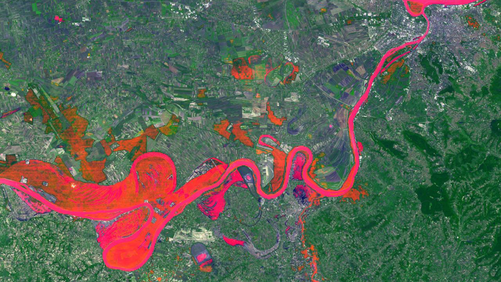
The fundamental problem is that floods and satellite observations are mismatched in time and space. Optical sensors often capture clouds rather than the floodwater beneath. Cloud-penetrating sensors like SAR can miss flood peaks if their orbital schedule doesn’t align with the event, and dense vegetation can obstruct floodwater from both optical and shorter-wavelength radar. Sensors with high temporal resolution typically deliver data at coarse spatial resolutions, sometimes tens of kilometers per pixel. These trade-offs form what we describe as the “iron triangle” of Earth observation: temporal resolution, spatial resolution, and cost. A sensor can typically be optimized for two, but rarely all three. Occasionally, the timing and conditions of a flood align well with sensors whose strengths are complementary across the iron triangle, yielding the kind of multi-sensor view shown in Figure 2.
Figure 2. Sentinel‐2 MSI True Color Image with Sentinel‐1 SAR derived flood‐extent superimposed on top. The top right circle highlights the missing SAR‐derived information, whereas the bottom circle highlights the missing optical information. Credit: Campo et al. [2026], Figure 5
What are some upcoming space-based sensor projects that could advance the field of hydrology?
Several are already reshaping the field. NISAR, a joint NASA–ISRO radar satellite launched in 2025, carries an L-band sensor designed to penetrate vegetation canopy, providing new insights into flooding beneath vegetation. Sentinel-1D, launched in late 2025, has restored the Sentinel-1 constellation to full two-satellite capacity, halving the revisit time. Landsat Next, a planned three-satellite constellation with 26 spectral bands and a six-day revisit, would provide valuable hydrologic data at both high temporal and spectral resolutions. However, recent budget pressures have introduced uncertainty about its final scope. Finally, the HydroGNSS mission from ESA will use GNSS-R to monitor hydrologically linked Essential Climate Variables.
Editor’s Note: It is the policy of AGU Publications to invite the authors of articles published in Reviews of Geophysics to write a summary for Eos Editors’ Vox.
Citation: Campo, C. (2026), Can any single satellite keep up with the world’s floods?, Eos, 107, https://doi.org/10.1029/2026EO265016. Published on 20 April 2026.
This article does not represent the opinion of AGU, Eos, or any of its affiliates. It is solely the opinion of the author(s).
Editors’ Vox is a blog from AGU’s Publications Department.
Mesoscale and submesoscale ocean processes influence ocean circulation, air-sea fluxes, ecosystem variability, and transport of materials. A new article in Reviews of Geophysics examines how these fine-scale processes shape the Indian Ocean, an ocean basin with unique monsoon behavior and a disproportionate impact on global climate. Here, we asked the authors to explain what mesoscale and submesoscale processes are, the techniques an
Mesoscale and submesoscale ocean processes influence ocean circulation, air-sea fluxes, ecosystem variability, and transport of materials. A new article in Reviews of Geophysics examines how these fine-scale processes shape the Indian Ocean, an ocean basin with unique monsoon behavior and a disproportionate impact on global climate. Here, we asked the authors to explain what mesoscale and submesoscale processes are, the techniques and challenges of observing and modeling fine-scale processes, and how biogeochemical cycles and climate change interact with these processes.
In simple terms, what are mesoscale and submesoscale processes?
Mesoscale processes pertain to oceanic features such as eddies and fronts, which typically span a range of approximately 10 to 100 kilometers and can persist from weeks to months. Submesoscale processes are of an even smaller scale, ranging between approximately 100 meters and 10 kilometers, and evolve rapidly within a time frame of hours to days. These encompass sharp fronts, filaments, and small vortices.
Mesoscale processes account for more than 80% of the total kinetic energy. Submesoscale motions are of particular significance as they generate robust vertical movements that establish a connection between the surface ocean and deeper layers. As elaborated in our review, mesoscale and submesoscale processes function as a crucial link between large-scale ocean circulation and small-scale turbulence, facilitating the transfer of energy across different scales and regulating the distribution of heat, salt, and nutrients throughout the ocean.
Why is it important to understand how fine-scale processes operate in the IndianOcean?
The Indian Ocean has a disproportionate influence on global climate.
The Indian Ocean has a disproportionate influence on global climate. It absorbs over a quarter of the ocean’s net heat gain and directly affects the environment and food security of nearly one-third of the world’s population. Unlike other ocean basins, the Indian Ocean is uniquely shaped by seasonally reversing monsoon winds and is strongly coupled with climate modes like the Indian Ocean Dipole and the Madden- Julian Oscillation. Mesoscale and submesoscale variability in this region modulates biogeochemical cycles, air-sea fluxes, and even large-scale energy balance. As our review highlights, understanding these fine-scale dynamics is essential for improving predictions of monsoon rainfall, tropical cyclone behavior, and long-term climate change.
How do scientists study mesoscale and submesoscale ocean processes?
Scientists employ a combination of field measurements, satellite observations, and numerical models, all of which were summarized in our review. In-situ observations serve as the foundation for mesoscale and submesoscale processes in the ocean. They encompass research cruises, moored arrays such as the RAMA network, Argo profiling floats, and autonomous platforms. The in-situ observations capture the three-dimensional structures and multiple variables during mesoscale and submesoscale processes.
Satellite altimetry has long been the principal tool for observing mesoscale eddies. However, the newly launched Surface Water and Ocean Topography (SWOT) mission is revolutionary, as it offers sea surface height measurements at an unprecedented resolution, enabling the direct observation of submesoscale features for the first time.
High-resolution regional models with grid spacings of a few kilometers or less enable researchers to simulate these processes and test dynamical theories under controlled conditions.
What are some of the challenges in observing and modeling these processes?
In our review paper, we tackled the challenges in observations by adhering to four principles, namely high-resolution (more observations in a relatively small region), synchrony (observations conducted at the same time), persistence (observations for a long time), and interdisciplinary (observations of multiple ocean properties). These principles are anticipated to offer valuable guidance for future observational endeavors to surmount the corresponding challenges.
Modeling also poses difficulties. Even state-of-the-art climate models are unable to explicitly resolve submesoscale processes. Consequently, their effects have to be approximated via parameterizations. The development of accurate parameterizations continues to be an active area of research. Moreover, as the model resolution improves, the widely employed hydrostatic approximation may lose its validity, necessitating more intricate non-hydrostatic formulations. Data assimilation for such rapidly evolving features presents a particularly arduous challenge.
How do fine-scale processes interact with biogeochemical cycles in the IndianOcean?
Mesoscale and submesoscale motions exert a strong regulatory influence on biogeochemical cycling.
Mesoscale and submesoscale motions exert a strong regulatory influence on biogeochemical cycling through the control of nutrient supply to the sunlit upper ocean. Cyclonic eddies elevate nutrient-rich deep waters into the euphotic zone, thereby promoting phytoplankton blooms. In contrast, anticyclonic eddies typically suppress surface productivity by deepening the mixed layer.
In the Arabian Sea, eddies and filaments can contribute up to 70% of the nutrients that support the monsoon-driven biological bloom. These fine-scale dynamics also have an impact on carbon dioxide exchange; mesoscale variability accounts for approximately 40% of the CO₂ flux variability in the western Arabian Sea. Moreover, eddies modulate oxygen minimum zones in the Arabian Sea and Bay of Bengal, where low oxygen levels have a profound effect on marine ecosystems.
How is climate change expected to influence these fine-scale processes in the Indian Ocean?
With the continuous progression of climate change, alterations in upper-ocean stratification, propelled by warming and modified freshwater inputs, are anticipated to transform the conditions giving rise to fine-scale instabilities. High-resolution climate model simulations suggest that in a warming global scenario, the eddy-active region associated with the Agulhas Current system may shift westward and poleward. This shift is correlated with the intensification of Agulhas leakage, which refers to the transport of warm Indian Ocean water into the Atlantic. These changes could exert far-reaching effects on global ocean circulation.
Warming is augmenting the frequency and intensity of marine heatwaves in the Indian Ocean.
Moreover, warming is augmenting the frequency and intensity of marine heatwaves in the Indian Ocean. These heatwaves disrupt vertical mixing and nutrient supply, thereby having cascading impacts on biological productivity. Nevertheless, substantial uncertainties persist in quantifying these long-term responses.
In general, there are two-way interactions between climate change and fine-scale processes. Alterations in one component will induce changes in the other, and the former will be subject to feedback from the latter.
What are the remaining questions or knowledge gaps where additional research is needed?
Our review reveals several key priorities. In the short term, specialized multi-scale observational campaigns are acutely required, especially in regions with insufficient sampling, to capture the three-dimensional structure and rapid evolution of submesoscale features. Additionally, a more in-depth understanding is needed regarding how eddies interact with barrier layers—regions characterized by strong salinity stratification that are unique to the northern Indian Ocean—and how these interactions regulate air-sea fluxes and marine heatwaves.
Longer-term challenges encompass integrating fine-scale dynamics into climate models and refining submesoscale parameterizations. Emerging tools from artificial intelligence and machine learning hold potential for representing unresolved processes and enhancing data assimilation. Finally, considering the logistical and financial requirements of fine-scale ocean research, sustained international collaboration will be indispensable.
Editor’s Note: It is the policy of AGU Publications to invite the authors of articles published in Reviews of Geophysics to write a summary for Eos Editors’ Vox.
Citation: Zhou, L., D. Wang, L. Wang, and C. Qiu (2026), Small-scale Indian Ocean dynamics underpin marine ecology and climate, Eos, 107, https://doi.org/10.1029/2026EO265025. Published on 4 June 2026.
This article does not represent the opinion of AGU, Eos, or any of its affiliates. It is solely the opinion of the author(s).
Editors’ Highlights are summaries of recent papers by AGU’s journal editors.
Source: Space Weather
TianQin is a geocentric space-borne gravitational wave detector, which is proposed to detect the gravitational wave by measuring tiny displacements using inter-satellite laser interferometry. However, the space surrounding the orbit and laser links of TianQin is not a vacuum—but filled with plasma, which can bend the laser links and induce pointing accuracy noise in the gravitational wave de
TianQin is a geocentric space-borne gravitational wave detector, which is proposed to detect the gravitational wave by measuring tiny displacements using inter-satellite laser interferometry. However, the space surrounding the orbit and laser links of TianQin is not a vacuum—but filled with plasma, which can bend the laser links and induce pointing accuracy noise in the gravitational wave detection.
Based on a global magnetohydrodynamic model, Zhou et al. [2026] use a ray-tracing method to obtain the laser deflection caused by laser propagation through plasma, and to evaluate the pointing accuracy noise. The result shows that the laser deflection effect caused by large-scale space plasma distribution under quiet to moderate space weather conditions does not represent a fundamental risk to the TianQin mission. However, during severe space weather events, the laser propagation effect could become a considerable noise in the gravitational wave detection.
This work establishes a connection between space weather and gravitational wave detection. Furthermore, this work raises awareness of the impact of space weather on other high-precision electromagnetic wave measurements in space.
Citation: Zhou, S. W, Su, W., Zhou, S. Y., Li, C. F., & Zhang, J. X. (2026). The pointing error due to laser propagation in space plasma for TianQin gravitational wave detection. Space Weather, 24, e2025SW004784. https://doi.org/10.1029/2025SW004784