Editors’ Highlights are summaries of recent papers by AGU’s journal editors.
Source: Journal of Geophysical Research: Earth Surface
Permafrost beneath Arctic roads is warming and becoming less stable, creating growing risks for northern infrastructure. Yet predicting how frozen ground will evolve remains difficult because subsurface conditions vary sharply over short distances, observations are sparse, and conventional process-based models are not easy to update as new field data arrive.
Source: Journal of Geophysical Research: Earth Surface
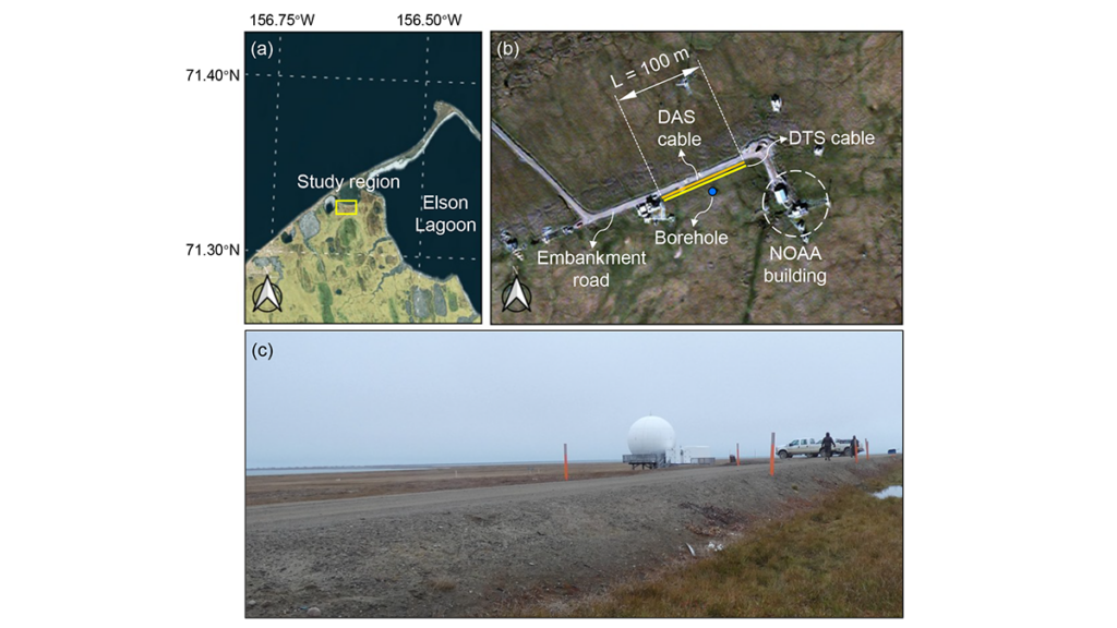
Permafrost beneath Arctic roads is warming and becoming less stable, creating growing risks for northern infrastructure. Yet predicting how frozen ground will evolve remains difficult because subsurface conditions vary sharply over short distances, observations are sparse, and conventional process-based models are not easy to update as new field data arrive. In a new study, Gou et al. [2026] address that challenge at an embankment road in Utqiaġvik, Alaska, using fiber-optic temperature measurements collected along a 100-meter transect to track how shallow ground conditions change through time. Rather than treating monitoring and modeling as separate tasks, the authors link them in a framework designed to evolve with the physical system itself.
What stands out here is not simply the use of machine learning, but the way the authors build a physics-informed digital twin for permafrost under infrastructure. Their framework embeds a neural network within a heat-transfer solver, so the governing physics remain central while the model can still update uncertain soil properties as new observations arrive. This study moves beyond black-box prediction toward an interpretable, updateable system that can reconstruct subsurface temperature fields, infer thermodynamic properties such as unfrozen water content and thermal conductivity, and then test those inferences against independent DAS data, borehole temperatures, and laboratory measurements. This makes the work more than a site-specific modeling exercise; it offers a credible pathway toward near-real-time permafrost forecasting and infrastructure monitoring in a rapidly warming Arctic.
Framework of the proposed digital twin model. The neural network (NN) takes soil temperature at each lateral position as input and outputs six unknown parameters that vary laterally with distance. These parameters are embedded in the heat‐transfer equation through constitutive relationships, and the resulting system is solved using a finite difference method (FDM). The difference between predicted and observed temperatures is computed and defined as “loss,” and the loss gradients are backpropagated to update the NN parameters. Credit: Gou et al. [2026], Figure 2
Citation: Gou, L., Xiao, M., Zhu, T., Martin, E. R., Wang, Z., Rocha dos Santos, G., et al. (2026). Physics-informed digital twin for predicting permafrost thermodynamic characteristics under an embankment road in Utqiaġvik, Alaska. Journal of Geophysical Research: Earth Surface, 131, e2025JF008787. https://doi.org/10.1029/2025JF008787
Editors’ Vox is a blog from AGU’s Publications Department.
The supply of magma from the Earth’s mantle is a primary source of heat to volcanic arc crust, where the heat is then dissipated through various processes. Much of this magmatic heat is dissipated as heated water, or aqueous fluid.
A new article in Reviews of Geophysics compares 11 different volcanic-arc segments where heat discharge via aqueous fluid has been well-inventoried to better understand the factors that influence this p
The supply of magma from the Earth’s mantle is a primary source of heat to volcanic arc crust, where the heat is then dissipated through various processes. Much of this magmatic heat is dissipated as heated water, or aqueous fluid.
A new article in Reviews of Geophysics compares 11 different volcanic-arc segments where heat discharge via aqueous fluid has been well-inventoried to better understand the factors that influence this process. Here, we asked the authors to give an overview of heat discharge from volcanic arcs, how scientists measure it, and what questions remain.
Why is it important to study how heat is dissipated from volcanic arcs?
The heat from these magmas matters for geothermal energy, patterns of groundwater flow, and the patterns of volcanic activity at the surface.
Volcanic arcs are the chains of volcanoes on top of subduction zones. They can produce some of Earth’s most explosive and hazardous eruptions. But much of the magma beneath the surface never erupts. Nevertheless, the heat from these magmas—and the simple fact of their existence and abundance—still matters for geothermal energy, patterns of groundwater flow, and the patterns of volcanic activity at the surface.
What are the main modes in which heat is discharged from volcanic arcs?
Heat at volcanic arcs can be carried by magmas, transmitted through the crust conductively, and carried by water seeping slowly through the crust. At the base of the crust, magmas are probably most important, with conduction coming in second. But as magmas move upwards through the crust, some of them solidify and impart their heat to their surroundings where it is transferred by conduction. Within a few kilometers of the surface, fluids seeping through the crust begin to take up all that heat, and so if we can quantify the heat carried by those fluids, we can retrace it to its origins in magmas.
How do scientists measure these different forms of heat loss?
Scientists measure the heat carried by erupting magmas using satellites, or by adding up the erupted masses and making an estimate of how much energy was released by cooling from eruption temperatures to solid igneous rocks at Earth’s surface. Conductive heat flow is measured by drilling holes in the Earth’s crust to see how quickly it gets hotter with depth.
Measuring the heat carried by aqueous fluids in the crust is in some ways the trickiest. One approach is to find all the springs where hot or even slightly warm water is trickling out and measure the temperature and discharge to estimate how much extra heat that water is carrying.
What are the challenges and uncertainties in measuring hydrothermal heat discharge?
One challenge is that many springs are only slightly warmer than you’d expect. There is good data for many hot springs, but there are data tracking these ‘slightly warm’ springs for only a subset of arcs. Another challenge is that warm underground fluids can flow laterally, so you have to try to account for that. This is not an uncertainty in hydrothermal discharge, but one additional big uncertainty for our study, where we were trying to quantify the proportion of magmas that freeze underground versus erupting, is in the estimates of how much magma has actually erupted through time.
What are some of the factors that influence hydrothermal heat loss?
A major goal of our paper is to try to quantify these hidden magmas.
A main factor that influences hydrothermal heat loss is the magmas that solidify underground. This link is the key motivation for our study. A major goal of our paper is to try to quantify these hidden magmas—how much magma needs to intrude the crust beneath the surface to supply the hydrothermal heat fluxes that we observe? The composition of magmas influences how much heat they can release. The depth at which magmas are emplaced also matters, because magmas that intrude the shallow crust eventually cool to lower temperatures than magmas emplaced in the lower crust and therefore release more heat.
What are the remaining questions or knowledge gaps where additional research efforts are needed?
A big outstanding challenge is combining estimates from hydrothermal data of how much magma is coming into the crust – like ours – with other approaches to estimating the same thing. The magmatic systems beneath volcanoes span the crust. At the base of the crust, you have magma supply, sort of like the water main feeding your plumbing system. Despite how fundamental magma supply is, we know remarkably little about it. It’s exciting to think about how the rates of magma supply could vary through time and space and why. Applying a range of techniques—including geophysical imaging, hydrothermal budgets, gas and igneous geochemistry, and petrology—to understand these questions could really be a game changer.
Editor’s Note: It is the policy of AGU Publications to invite the authors of articles published in Reviews of Geophysics to write a summary for Eos Editors’ Vox.
Citation: Black, B. A., S. E. Ingebritsen, and K. Sawayama (2026), Hydrothermal heat flow as a window into subsurface arc magmas, Eos, 107, https://doi.org/10.1029/2026EO265017. Published on 28 April 2026.
This article does not represent the opinion of AGU, Eos, or any of its affiliates. It is solely the opinion of the author(s).
In the winter of 923, a magnitude 7.5 earthquake struck the heart of Puget Sound. Shorelines slid into the water, the seafloor rose up, and a tsunami swept through the region.
The Seattle fault zone, actually a mesh of faults that runs right under its eponymous city, was responsible for this quake. The fault continues to pose one of the deadliest threats to the Pacific Northwest; if a similar quake were to hit today, it would threaten millions of lives and cause billions of dollars in damage
In the winter of 923, a magnitude 7.5 earthquake struck the heart of Puget Sound. Shorelines slid into the water, the seafloor rose up, and a tsunami swept through the region.
The Seattle fault zone, actually a mesh of faults that runs right under its eponymous city, was responsible for this quake. The fault continues to pose one of the deadliest threats to the Pacific Northwest; if a similar quake were to hit today, it would threaten millions of lives and cause billions of dollars in damage.
Two new papers dig into recurrence intervals, or the quiescent periods between earthquakes, for the Seattle fault zone. They offer good news and bad news: One study, published in Geology, found that in the past 11,000 years, the massive 923 event was the only quake of magnitude 7.5 or greater. The other study, published in GSA Bulletin, found that smaller, but still damaging, quakes occur more frequently than previously thought.
The new research indicates the worst-case scenario of frequent 923-style events is less likely than some scientists thought, said Harold Tobin, a geophysicist at the University of Washington and head of the Pacific Northwest Seismic Network, who was not involved in either study. But researchers also found that “the less worse, but still bad scenarios” are more likely than previously thought.
Meet the Seattle Fault
“For a fault that has had so much attention, there’s so much we still don’t know.”
The Seattle fault zone is a thrust fault system that stretches about 75 kilometers (46 miles) from the foothills of the Cascades east of Seattle to the Hood Canal, which runs along the shores of the Olympic Peninsula to the city’s west, passing under Seattle along the way.
Geologists began rigorously exploring the fault system in the early 1990s, intrigued by gravitational anomalies, uplifted marine terraces (stair-step geological formations along coastlines), and evidence of a roughly 1,000-year-old tsunami. All these features hinted at a major, shallow earthquake on a local fault zone—likely the 923 event.
But “for a fault that has had so much attention, there’s so much we still don’t know,” said Elizabeth Davis, an earthquake geologist at the University of Washington who led the Geology study.
The most pressing questions are how big quakes on the fault get, how often they hit, and, ultimately, what risks the fault poses to people who live in the Puget Sound area.
“It takes some real geologic sleuthing to get at those tough questions,” Tobin said.
Biggest Seattle Fault Quakes Are Rare
Davis focused on the activity of the main fault, which can generate the biggest quakes in the Seattle fault zone complex. It was responsible for the 923 quake. But the existing record went back only about 5,000 years.
“We just don’t know what the recurrence interval for these big quakes is,” Davis said. “We wanted to lengthen the record.”
To do so, Davis and her collaborators turned to marine terraces, the oldest of which date back to the end of the last ice age about 11,000 years ago. The quake in 923 raised terraces by about 8 meters (26 feet), and scientists wanted to look for similar-scale uplift in terraces all around the sound.
The researchers mapped more than 150 terraces around Puget Sound and measured their depths. After accounting for regional slopes, they estimated uplift over time that could have been caused by quakes.
They found that in that 11,000-year period, only the 923 event generated significant uplift. Thick sediment mantles could mask smaller events but not 923-scale quakes, Davis said.
Estimating true recurrence intervals requires knowing the timing of multiple events. But the finding is “not bad news,” she said. It provides some evidence that the recurrence interval is likely not shorter than about 5,000 years.
“That could give us more of a buffer between now and when the next big one like that will happen,” said Stephen Angster, a U.S. Geological Survey geologist who led the GSA Bulletin study.
Smaller, Damaging Quakes Are More Frequent
Angster’s work focused on Seattle’s secondary faults, which are smaller, mostly blind faults (those not visible at the surface) capable of generating damaging earthquakes. Previous work had shown that one of these secondary faults generated a magnitude 6.7 earthquake, highlighting the risk they pose. Angster wanted to explore rupture histories of these secondary faults, particularly whether they could rupture independently from the main fault.
The researchers used a suite of paleoseismic tools, including magnetic data, field and lidar mapping, trenches dug across faults, and geochronology. They studied two newly identified secondary faults that have orientations similar to the main fault.
They found three new earthquakes to add to the region’s seismic history, including the oldest and youngest events in the known record, which were around 11,000 years ago and in the early 1800s, respectively. The earthquakes appear to be evidence of ruptures that occurred independently of the main fault, suggesting that the smaller—but still dangerous—secondary faults should be considered in hazard modeling.
With that lengthened record and the addition of three quakes, the recurrence interval the researchers found was about every 350 years over the past 2,500 years. This timing refined the previous estimate of every several hundred years.
There also appears to be an increase in activity over the past 2,000 years.
“Maybe we should be paying attention to that,” Angster said.
What Happens Next
“There are other earthquakes that aren’t as big but that occur more frequently. Those might not be as catastrophic, but it would be a very bad scenario for Seattle” if such events occurred.
“These are both carefully done studies,” Tobin said. “We now have evidence that the 923 event was the biggest in 11,000 years. But there are other earthquakes that aren’t as big but that occur more frequently. Those might not be as catastrophic, but it would be a very bad scenario for Seattle” if such events occurred.
It’s still to be determined whether the risk from secondary faults will be incorporated into the National Seismic Hazard Model, which includes the 923 quake but not smaller ones along the Seattle fault zone. The secondary faults were left out in previous efforts because they are shorter than the minimum length required to be included and because of uncertainties in their potential rupture magnitude.
Citation: Dzombak, R. (2026), On the Seattle Fault, the biggest quakes aren’t the most likely, Eos, 107, https://doi.org/10.1029/2026EO260114. Published on 14 April 2026.
A critical ocean current that regulates Antarctica’s climate may have formed only once continents separated and winds aligned with new ocean passageways, according to a new study published in the Proceedings of the National Academy of Sciences of the United States of America.
Today, the Antarctic Circumpolar Current transports more than 100 times as much water as all of Earth’s rivers combined and, critically, insulates the Antarctic Ice Sheet from heat at lower latitudes. A clear picture of
Today, the Antarctic Circumpolar Current transports more than 100 times as much water as all of Earth’s rivers combined and, critically, insulates the Antarctic Ice Sheet from heat at lower latitudes. A clear picture of the origins of this current can help scientists further understand the relationships between contemporary ocean dynamics, the global climate, and ice formation in Antarctica.
“It’s very interesting to learn more about this current, how it developed, and what role it played in the climate change that was happening at that time,” said Hanna Knahl, a paleoclimatologist and doctoral student at the Alfred-Wegener-Institut in Germany and lead author of the new study.
The Birth of a Current
About 34 million years ago, Earth was undergoing a climatic shift, now known as the Eocene-Oligocene transition, during which atmospheric carbon dioxide decreased and the planet cooled.
Earth’s tectonic plates in the Southern Ocean moved away from each other, opening and deepening bodies of water such as the Tasmanian Gateway and the Drake Passage, which separate Antarctica, Australia, and South America.
For years, scientists hypothesized that the alignment of these newly formed waterways, along with westerly winds, could have channeled ocean water and spurred the formation of the Antarctic Circumpolar Current.
“The exact position of the westerly winds and their relative position to the [ocean] gateways have to click together.”
To test that hypothesis, Knahl and her colleagues simulated conditions of the early Oligocene Southern Ocean with a coupled model that included ocean dynamics, atmosphere and wind patterns, temperatures, ice sheet growth, and precipitation. The research team compared these simulations to data from actual Antarctic sediment cores and scans of the ocean floor.
Results confirmed that westerly winds were necessary for the Antarctic Circumpolar Current to form.
“The exact position of the westerly winds and their relative position to the [ocean] gateways have to click together,” Knahl said.
Joanne Whittaker, a marine geophysicist at the University of Tasmania who was not involved in the new study, was a coauthor of a 2015 study that proposed westerly wind alignment played a role in the formation of the current. Knahl’s study presents a more sophisticated model of the early Oligocene Southern Ocean and is a great next step in the investigation of the current’s origins, Whittaker said.
“They did a really nice job of taking a range of different people’s work and linking it all together,” she said.
Oligocene Understandings
“If you can have a model that works in the past, it’s going to give you confidence that it’s going to work for the future, as well.”
Scientists often use Earth’s past behavior to better understand how Earth systems may behave in the present or future. “If you can have a model that works in the past,” Whittaker explained, “it’s going to give you confidence that it’s going to work for the future, as well.”
The Eocene-Oligocene transition is a key to understanding the relationship between atmospheric carbon, ocean dynamics, and the glaciation of Antarctica, Whittaker said. Knowing how the current’s behavior affected carbon uptake millions of years ago helps scientists model how the present current’s behavior might also affect atmospheric carbon.
In addition to carbon uptake, the new research hints at how changes in westerly winds may influence the advance and retreat of the Antarctic Ice Sheet. Some modeling and proxy data indicate the westerly winds that spurred the Antarctic Circumpolar Current’s formation 34 million years ago have shifted in the past century and may continue to shift in the future. Understanding the role these winds initially played in the current’s development may shed light on the current’s present ability to guard the Antarctic Ice Sheet from warmer air masses.
There are still Oligocene patterns that require more research to sort out, though. For example, modeling in the new study showed interesting asymmetries in the timing of the development of different parts of the Antarctic Circumpolar Current, Knahl said. Scientists know from proxy data and modeling that similar asymmetry exists in the history of the Antarctic Ice Sheet; the ice sheet in East Antarctica began to form about 7 million years before the ice sheet began to form in West Antarctica.
“It could be interesting to see if there’s a connection between the asymmetries that we see here,” Knahl said. “Are they linked, or were they more or less independent?”
Citation: van Deelen, G. (2026), Widening channels and westerly winds together formed Earth’s strongest current, Eos, 107, https://doi.org/10.1029/2026EO260126. Published on 24 April 2026.
Editors’ Highlights are summaries of recent papers by AGU’s journal editors.
Source: Journal of Geophysical Research: Solid Earth
Highly porous rocks, such as sandstones, often deform in a surprising way: instead of breaking apart or sliding, they develop thin zones called deformation bands. In these bands, the grains are squeezed closer together, making the rock denser, and reducing how easily fluids such as water or oil can move through it. This behavior is important because it affects
Source: Journal of Geophysical Research: Solid Earth
Highly porous rocks, such as sandstones, often deform in a surprising way: instead of breaking apart or sliding, they develop thin zones called deformation bands. In these bands, the grains are squeezed closer together, making the rock denser, and reducing how easily fluids such as water or oil can move through it. This behavior is important because it affects both the strength of rocks and their ability to store and transport fluids underground. However, these bands are difficult to model because they form suddenly from an initially uniform material and concentrate deformation into very narrow zones.
Wang et al. [2026] developed a computer modeling approach called a “phase‑field model” to study this process. Instead of drawing the bands in the initially homogeneous rock, the model allows them to appear naturally as the system evolves and minimizes its energy. The study shows how grain crushing and rearrangement allows the formation of localized deformation zones. The results also demonstrate that natural spatial variations in the rock, such as differences in grain size or porosity, strongly influence where bands initiate and how they grow. Additionally, the model captures how deformation changes from sliding (shear bands) to pure compaction as pressure increases. Overall, this work provides a realistic way to understand how localized deformation develops in rocks, with important implications for geology, engineering, and energy applications.
Citation: Wang, Y., Zhang, C., Braun, P., Kang, X., & Wu, W. (2026). How does heterogeneity control strain localization patterns in high-porosity rocks? Journal of Geophysical Research: Solid Earth, 131, e2025JB032494. https://doi.org/10.1029/2025JB032494
For roughly 45 million years, the eastern section of the African continental plate has been slowly pulling apart. Like a giant zipper extending from the Red Sea to Mozambique, the East African Rift System will likely be home to new oceanic crust that will well up from the widening split in Earth’s surface. While most of the rifts in that system are still zipped shut, the Afar region in northern Ethiopia has already partially unzipped and may be starting to create a future ocean basin.
Most m
For roughly 45 million years, the eastern section of the African continental plate has been slowly pulling apart. Like a giant zipper extending from the Red Sea to Mozambique, the East African Rift System will likely be home to new oceanic crust that will well up from the widening split in Earth’s surface. While most of the rifts in that system are still zipped shut, the Afar region in northern Ethiopia has already partially unzipped and may be starting to create a future ocean basin.
Most models of this rift system suggest that it should continue to unzip sequentially from north to south. However, new research suggests that a region in the middle of the zipper is on the verge of splitting open.
High-resolution seismic reflection data show that the crust near Kenya’s Lake Turkana is only 13 kilometers thick. This suggests that the region has entered the second stage of rifting, called necking, and is one step closer to breaking apart. It is the only rift zone on Earth currently undergoing this short-lived tectonic process.
The Lothagam site in the Turkana Rift Zone contains tilted sediments from the late Miocene (about 7 million years ago), just before the necking phase of rifting commenced. Credit: Christian Rowan
Breaking Up Is Hard to Do
Just like mid-ocean ridges on the seafloor, sections of Earth’s crust on land also stretch apart as tectonic plates separate. This process, called rifting, takes place in three stages. First, the crust stretches, creating tension. Then it rapidly thins like pulled taffy—this is the necking stage. Finally, magma wells up from the lithospheric mantle, which creates new seafloor and breaks the continental plate apart.
“This is one of the unique places on Earth where you can see a continental rift.”
Not every rift makes it that far. Some remain stuck in the stretching phase with crust more than 20 kilometers thick. But northern sections of the East African Rift System (EARS), specifically the Afar Rift and the Red Sea, are already undergoing the final stage, oceanization.
“This is one of the unique places on Earth where you can see a continental rift,” said Anne Bécel, a geophysicist at Lamont-Doherty Earth Observatory of Columbia University in Palisades, N.Y., and coauthor of new research published in Nature Communications in April. “The East African Rift System has been studied for a very long time by geologists to really learn about our planet and how continents break apart, and then transpose that to mid-ocean ridges where oceanic plates spread apart.”
The team suspected that the Turkana Rift Zone, located at a critical triple junction in northern Kenya, was behaving differently from other areas of the rift system. It is home to an unusually large and continuous hominin fossil record dating back about 4 million years. Past research has also shown that the bottom of the crust, called the Moho, is unusually shallow in the Turkana Basin, just 20 kilometers deep compared with the average depth of 39 kilometers farther away from the rift.
During several field expeditions to Lake Turkana in partnership with local industries, the team mapped the top of the continental crust using borehole measurements and seismic reflection—sending seismic waves into the ground and measuring how the waves bounce back, like sonar. They combined those measurements with past research into Moho depths to calculate the crustal thickness near Lake Turkana.
That map showed that far away from the rift, the crust is more than 35 kilometers thick, but in the Turkana Rift Zone it is a mere 13 kilometers thick, below the threshold for necking.
“If you look at the modern day topography, the whole East African Rift is in this really low, broad land between two big plateaus, one to the north in Ethiopia and one towards the south,” said lead researcher Christian Rowan, a geologist and doctoral candidate at Columbia University. “It’s this very strange topographic feature, and part of that low-lying topography is actually how thin the crust is there.”
“The oldest rocks that record the initiation of the East Africa Rift System are also in the Turkana Rift,” said coauthor Folarin Kolawole, a Columbia University geologist. Geochemical analysis of those rocks suggests that necking in the Turkana Rift Zone began about 4 million years ago.
Christian Rowan measures a fault in the Turkana Rift. Credit: Christian Rowan
About to Break?
“Any time you have a place on the planet that is rare in the modern but seen in the past, it is compelling,” said Erik Klemetti Gonzalez, a volcanologist at Denison University in Granville, Ohio, who was not involved with this research. “The data does show that the Turkana Rift is the home of anomalously thin continental crust, so if you are looking for a location that meets criteria for necking, it seems to be the case.”
The team suspects that Turkana might have been primed to split apart more easily because another rifting event took place there a mere 17 million years before the present rift began. The Turkana Basin inherited a weaker section of crust that didn’t have time to fully heal in the (geologically) short time between rifting events. There was also an extended period of magmatic activity throughout much of the past 45 million years.
“Magmatism is well known to be a significant weakening factor in rifting,” Rowan said. “I think the two compounding effects of this inheritance and then magnetism is why the Turkana rift is so much more mature than other segments.”
“I would hope that more collaboration with African geoscientists could create the ability to collect data from places that have been more inaccessible over the past half century.”
“There are many ‘failed rifts’ in the geologic record, so the question of whether the EARS is actually leading to a continental break up, albeit a small one, is still very much up in the air,” Klemetti Gonzalez said. These new results tip the scales toward breakup, but he noted that more of the rift system still needs to be mapped to really understand the fate of this region.
“I would hope that more collaboration with African geoscientists could create the ability to collect data from places that have been more inaccessible over the past half century,” he added.
Rowan and his team are working toward that end by continuing to map crustal thicknesses in other nearby rift zones.
“This was the only known rift that was undergoing necking along the entire East African Rift System, or in the world,” said Kolawole. “But based on ongoing work, there is evidence that there are other segments that are at the onset of necking in the East African Rift System.”
Citation: Cartier, K. M. S. (2026), Eastern Africa is splitting apart, but not where we expected, Eos, 107, https://doi.org/10.1029/2026EO260148. Published on 12 May 2026.
Seeking Solutions to PFAS Pollution
Chemical Companies Are Churning Out New PFAS. Where in the World Are They Ending Up?
The Persistence of PFAS
A Peculiar Polymer Paired with Sunlight Could Remove PFAS
Tracing the Path of PFAS Across Antarctica
Pollution Is Rampant. We Might As Well Make Use of It.
On a rocky archipelago in the North Atlantic Ocean, staff at the Faroese Environment Agency and the Faroe Marine Research Institute regularly sample tissues from the North At
On a rocky archipelago in the North Atlantic Ocean, staff at the Faroese Environment Agency and the Faroe Marine Research Institute regularly sample tissues from the North Atlantic long-finned pilot whales that roam the waters around the islands. The archive of these samples stretches back to the 1980s and has helped researchers determine the reach of human-made contaminants in the remote marine environment.
Jennifer Sun is one of those researchers. Sun studies PFAS—per- and polyfluoroalkyl substances, commonly known as “forever chemicals”—at Harvard University and is the lead author of a recently published study that analyzed how these toxic chemicals have accumulated in pilot whale tissue over the past 2 decades.
Using samples of whale tissue collected between 2001 and 2023, Sun and her colleagues measured a parameter called bulk extractable organofluorine, which shows the overall amount of organofluorine-containing chemicals (including PFAS) in the tissue. They then used a more targeted analysis able to confirm the identity of 28 specific chemicals out of thousands of possible PFAS formulations.
The pilot whale tissue showed an expected decrease in the concentrations of older PFAS but an unexpected scarcity of newer PFAS chemicals. Credit: Jennifer Sun
The study’s results showed an expected decrease in the concentrations of older PFAS but an unexpected absence of newer PFAS chemicals. This anomaly could be indicative of an emerging question in PFAS research: Where are the newest PFAS going?
Prolific PFAS
There are two general categories of PFAS. The first includes legacy PFAS such as perfluorooctanoic acid (PFOA) and perfluorooctane sulfonic acid (PFOS). Chemical manufacturers produced these compounds in the 1970s, 1980s, and 1990s for products including nonstick cookware and food packaging and in industries such as fabric waterproofing, industrial manufacturing, and firefighting.
Legacy PFAS were phased out in the early 2000s, and novel PFAS were made to replace them. The term “novel” is independent of chemical properties and instead refers to when the chemicals’ production began, though novel PFAS typically have formulations meant to reduce their persistence in the environment. For example, many novel PFAS molecules have shorter chains of fluorinated carbons than their legacy counterparts.
Novel PFAS include possibly millions of different chemical structures, and their production and use are increasing globally.
A generic PFAS molecule includes a compound head connected to a tail of fluorinated carbons. Older PFAS generally have longer tails (seven or eight carbons) than newer ones. Credit: Mary Heinrichs/AGU, after https://bit.ly/pennstate-ext-pfas
In the United States and elsewhere, regulatory structures that limit PFAS production target specific chemicals, such that every new formulation by a company must be tested individually before restrictions are put in place. With companies continually conjuring new PFAS formulations—which environmental advocates often call “regrettable substitutions” for their sometimes harmful effects—understanding the fate and transport of novel PFAS is difficult and time-consuming. Research on the behavior of specific PFAS may be a drop in the bucket when millions of potential PFAS, with millions of potential behaviors, pose current and future risks to people and the environment.
Scientists like Sun are determined to untangle how the fate of these new chemicals differs from their predecessors. As Sun expected, the phaseout of legacy PFAS was reflected in the pilot whale tissue she tested. These results are good news; they clearly show that the bans on legacy PFAS are working.
“We’re still finding [older] compounds, but clearly, they are no longer as abundant in the environment as they used to be, which is a positive,” said Bridger Ruyle, an environmental engineer at New York University who studies PFAS and assisted Sun and her coauthors in deciding which methods to use for the new study.
But Sun and her colleagues also expected an overall increase in concentrations of novel PFAS—after all, production of these chemicals is higher than ever, and researchers finally had the analytical tools to catch them.
“The inference is, if it’s not in the whales, and it’s not in the ocean…where is it?”
That wasn’t what they found. Instead, all but two of the emerging PFAS they tested for were virtually nowhere to be seen in the whale tissue, leaving the scientists leading the study to wonder where novel PFAS were accumulating or if instrumentation was limiting their detection.
“We do know that the novel PFAS are being produced, which means they’re going somewhere. Where they are, and how exposed people and other wildlife are, is not as clear,” Sun said.
“The inference is, if it’s not in the whales, and it’s not in the ocean…where is it?” asked Elsie Sunderland, an environmental scientist at Harvard University and coauthor of the new study.
Sun and Sunderland’s question—asking where novel PFAS are going—is one scientists are probing from multiple angles. Those who study particle transport are asking how novel PFAS might travel through Earth’s water and air. Those on the chemistry side of the investigation are deducing how novel PFAS might break down. And those who monitor environments are looking for traces of novel PFAS in various corners of Earth.
The answers to their questions have direct, practical implications for human and environmental health and could indicate whether a growing proportion of harmful PFAS may be ending up in close proximity to humans—where we work and eat and breathe.
A Toxic Legacy
The chemical properties of PFAS have made the chemicals useful since the 1940s. These same properties also make them highly persistent—the most durable types may not break down in the environment for several thousand years.
PFAS are linked to certain cancers and other human health harms. Much of the available data linking PFAS to poor health come from analyses of legacy PFOA and PFOS. They show an association between increased exposure to these chemicals and altered immune and thyroid function, liver and kidney disease, reproductive system disruptions, and more.
Chemical manufacturers phased out production of legacy PFAS after scientific evidence emerged associating PFAS and human health harms, businesses began to lose money in massive lawsuits, and regulations tightened. Novel PFAS were intended to show properties similar to legacy PFAS but were meant to break down more easily in the environment (lower persistence) and accumulate less easily in living tissue (lower bioaccumulative ability), though studies have shown mixed results about whether novel PFAS are actually safer for humans or break down more easily.
Because PFAS production data are often proprietary, scientists who study PFAS, like Sun, must rely on partial inventories of PFAS production or reverse-engineer those numbers from observations in the environment.
“We call it chemical Whac-A-Mole.”
Without a clear list of the chemical structures of novel PFAS, scientists don’t always have the analytical standards necessary for routine detection. And once scientists do understand the behavior of a PFAS chemical, it may be quickly replaced by another, unknown alternative. “We call it chemical Whac-A-Mole,” Sunderland said.
Legacy PFAS tend to have a high affinity for water and typically end up in the ocean, the place scientists refer to as the chemicals’ “terminal sink.” Many legacy PFAS also entered the ocean through atmospheric transport such as rain or snow. But because of the sheer number of chemical formulas and the chemical differences between legacy and novel PFAS, the pathways that novel PFAS take through the environment are less clear.
Tracking the movement and accumulation of novel PFAS in the environment is crucial for understanding how these chemicals may affect ecological and human health.
Still, the science is inconclusive about whether novel PFAS are moving or accumulating differently than their legacy counterparts, whether they have a different terminal sink, and where that terminal sink may be.
Close to Home
One possible answer to the question of the missing novel PFAS may have to do with geography. The chemicals may not have reached pilot whales in the Faroes because something about the new chemistry has led them elsewhere in the environment. To Sun, evidence suggests “that a lot of these novel PFAS, which we know are being produced, may not be transporting out into this more remote environment either at all or as quickly.”
Novel PFAS might be accumulating closer to their sources—and closer to us. “It may simply be that some of the replacement PFAS don’t make it all the way out into the open ocean. But if they are still in the terrestrial environment and the near-coastal environment, then wildlife and people who live close to the sources can be exposed, said Frank Wania, an environmental chemist at the University of Toronto Scarborough.
For example, one study monitored PFAS in coastal beluga whales in Canada’s St. Lawrence Estuary, relatively close to human communities and PFAS manufacturing sources. The study showed increasing concentrations of unregulated novel PFAS in whale tissue from 2000 to 2017, while concentrations of legacy PFAS declined.
The suggestion that novel PFAS are accumulating close to human communities is supported by measurements of PFAS in human tissue, too. Studies show that a high proportion of detectable organofluorine chemicals in human tissue are increasingly unidentifiable, suggesting that some of the novel PFAS production “is in us,” Sunderland said.
Far and Away
Though there are some indications that novel PFAS may be retained closer to human communities, there are also reasons to think some novel PFAS chemistries have resulted in substances that can actually travel farther and more easily than their legacy counterparts.
Anna Kärrman, an environmental chemist at Örebro University in Sweden, said that some novel PFAS may be more easily transported in the environment: “The more novel chemistries are increasing the properties of being very mobile in water, very mobile in the atmosphere, and not necessarily very bioaccumulative.”
The mobility of novel PFAS was on full display in a 2020 study that Sunderland coauthored, in which researchers reported detecting hexafluoropropylene oxide-dimer acid, a novel PFAS chemical more commonly known as GenX, in the Arctic for the first time. GenX, produced by chemical manufacturer Chemours, was meant to replace the legacy compound PFOA. The 2020 study suggested GenX “has already moved quite a bit,” said Rainer Lohmann, a marine geochemist who leads the STEEP (Sources, Transport, Exposure and Effects of PFAS) Center at the University of Rhode Island.
A pulley system mounted on a red beam pulls a small envelope filled with water along a string. Credit: Thomas Soltwedel
The 2020 study also found higher concentrations of PFAS in the Arctic Ocean’s surface water, suggesting that the atmosphere was a particularly important transport pathway for chemical transport. This idea is supported by studies of High Arctic ice caps, which experience contamination only from atmospheric sources, and polar bear tissue. Atmospheric transport of novel PFAS is a subject “at the edge” of PFAS research, Sunderland said.
Wherever researchers look, they’re finding that atmospheric transport is an important pathway by which some PFAS, especially PFAS precursors—chemicals that break down in the environment and become PFAS (either novel or legacy)—move. One idea called the PAART (precursor atmospheric and reaction transport) theory was developed by Scott Mabury, an environmental chemist at the University of Toronto, and others. The PAART theory proposes that many of the harmful PFAS that end up in the most remote parts of Earth are the result of the breakdown of volatile precursor PFAS that have traveled in the atmosphere.
According to Lohmann, atmospheric transport means the ocean remains a terminal sink because many novel PFAS transported in rain or snow will ultimately be deposited in the ocean.
In this scenario, the question of why novel PFAS are not bioaccumulating in Faroese pilot whales remains a mystery. While Lohmann suggests the novel compounds simply don’t accumulate in living tissue, Sunderland isn’t sure that’s the whole story: “As apex predators, the whales are sentinels for what is available and being taken up from the ocean,” she wrote in an email. “Since we don’t see [novel PFAS], it seems unlikely there are large quantities of these chemicals present.”
Profuse PFAS
Another possible explanation for the surprising results of Sun’s whale study could be that there’s just a lag; that is, novel PFAS will end up in Faroe Island pilot whales someday but haven’t yet. Chemicals that could eventually end up in the ocean may be temporarily trapped in soils or recycled back into terrestrial ecosystems via sea spray aerosols, for example.
“The delay we are seeing in the ocean response may in fact be [PFAS] precursors being retained in source zones,” Sunderland wrote in an email. These chemicals may be “taking a really long time to be transformed into more mobile compounds.”
In their pilot whale study, Sun and her colleagues modeled the transport of PFAS to the subarctic and found a 10- to 20-year lag existed between the production of a legacy PFAS compound and its detection in whale tissue. We’re still within that range for many novel PFAS. Sun said she would have expected them to show up in pilot whale tissue by now if they behaved like their legacy counterparts, though it’s possible that it has taken time for the volume of novel PFAS production to ramp up, increasing the time it would take for the substances to be detected in tissues.
The anomaly documented in the pilot whale study has led researchers to call for more investigation (and perhaps greater regulation) of novel PFAS. Credit: Bjarni Mikkelson
Still, the number of possible novel PFAS chemistries—again, there could be several million different compounds—makes it difficult to generalize how these new substances are, as a group, moving through the environment. “Because the exact structures of all [novel] PFAS remain unknown, some compounds may simply not be captured by the methods used,” Heidi Pickard, an environmental engineer at the consulting firm Ramboll and coauthor on the new whale study, wrote in an email.
Another reason novel PFAS are harder to study is that companies release lower concentrations of more kinds of the chemicals, rather than the “monstrously high” emissions of some legacy PFAS in the 1970s–1990s, noted Mabury, who was not involved in the new pilot whale study.
A New Regulatory Approach
According to Sun and Sunderland, cataloging differences between novel and legacy PFAS misses the broader point: We simply need to produce less PFAS. We’ve known for decades that PFAS harm human health, and some scientists have even argued that humans’ continual production and release of novel chemical compounds could drive Earth beyond a “safe operating space.”
“Researchers are critical for exposing the problem. But that, to me, is not the central issue here. The central issue here is a societal issue.”
Where scientists probe next may be less urgent than how policymakers decide to tackle the PFAS problem, Sunderland said: “Researchers are critical for exposing the problem. But that, to me, is not the central issue here. The central issue here is a societal issue.”
Chemical manufacturers are actively creating novel PFAS all the time. Kärrman, for example, has noticed patent applications for PFAS compounds with chemistries that “are nothing like we have seen before” that may start entering our environment in 5 or 10 years.
To Kärrman, that’s a reason for governments to push for chemical regulation based on properties such as persistence and bioaccumulation, rather than the chemical-by-chemical formula used in most countries, including the United States.
Such an approach has gotten traction in Europe via a proposal by the European Chemicals Agency to restrict the entire class of PFAS chemicals. The proposal is still under evaluation, and a final decision is expected by the end of the year.
In the United States, PFAS regulation and remediation are a key aspect of the Trump administration’s Make America Healthy Again movement, according to the EPA, and the federal government and some states already limit the concentrations of individual PFAS in drinking water. However, the EPA also said it planned to weaken some of those limits last year.
“We’re in a cycle of picking these regrettable alternatives [to legacy PFAS] and then figuring out that it was regrettable decades later,” Sunderland said. “We’re never going to catch up using this chemical-by-chemical approach.”
Citation: van Deelen, G. (2026), Chemical companies are churning out new PFAS. Where in the world are they ending up?, Eos, 107, https://doi.org/10.1029/2026EO260136. Published on 30 April 2026.
Tiny saltwater channels have a big influence on sea ice.
Sea ice typically includes pockets or channels of brine that allow salt water to flow vertically through the ice. When those channels align neatly, they need to make up only about 5% of the ice volume before the water can flow. But in more disordered, granular ice, salt water starts to flow only when the brine channels take up more space—roughly 10% of the ice volume, according to a new study published in Scientific Reports.
“If we’
Tiny saltwater channels have a big influence on sea ice.
Sea ice typically includes pockets or channels of brine that allow salt water to flow vertically through the ice. When those channels align neatly, they need to make up only about 5% of the ice volume before the water can flow. But in more disordered, granular ice, salt water starts to flow only when the brine channels take up more space—roughly 10% of the ice volume, according to a new study published in Scientific Reports.
“If we’re trying to find predictive models about how these ice cores are responding under climate change, it’s going to be necessary to take into account these structural and microstructural conditions.”
This higher threshold could slow the drainage of surface melt ponds, as well as the transport of nutrients to microbial communities inside the ice.
“If we’re trying to find predictive models about how these ice cores are responding under climate change, it’s going to be necessary to take into account these structural and microstructural conditions,” said Stephen Ackley, a sea ice researcher at the University of Texas at San Antonio who was not involved in the study.
Disorderly Constructs
As seawater freezes, it forms a mixture of ice crystals and brine. In calm conditions, the ice slowly grows into long, parallel crystals separated by orderly brine channels. This columnar sea ice is common in the Arctic, and its properties have been widely used in sea ice models.
But in choppy waves or when the ice’s snow-covered surface floods and refreezes, new ice can’t grow into these ordered columns. Instead, it forms small, randomly oriented grains separated by more complex pores containing brine and gases. Called granular ice, this form is more common in Antarctica but is becoming increasingly prevalent in the Arctic as temperatures rise and ice cover thins.
“It’s the sequel we’ve been waiting decades for.”
In 1998, University of Utah mathematician Kenneth Golden established the first estimate of the point at which the brine channels are connected enough to allow water to flow in columnar ice, called the percolation threshold. The new work, also led by Golden, extends a similar analysis to granular sea ice.
“It’s the sequel we’ve been waiting decades for,” said Don Perovich, a sea ice researcher at Dartmouth who was not involved in the new work.
To quantify the percolation threshold for granular ice, Golden and his colleagues collected sea ice samples during two expeditions off the eastern coast of Antarctica in 2007 and 2012. They measured how quickly water moved through the brine channels in the ice. After the 2012 expedition, they also mapped the arrangement of ice crystals within the ice blocks to correlate those permeability measurements with the microscale structure of the ice.
Most climate models are based on the assumption that the microstructure of sea ice is organized into columns, like those in the image on the left. But new research shows that granular ice, as seen on the right, is growing more common in the Arctic, which could affect climate modeling. Credit: Golden et al., 2026, https://doi.org/10.1038/s41598-026-41706-w, CC BY-NC-ND 4.0
The finding that in granular ice, about twice as much of the ice volume needs to be brine for water to flow compared to columnar ice suggests that brine channels within granular ice are much less interconnected.
With the higher threshold, “you have to reassess all these models, anything that relies on fluid flow through sea ice,” if granular ice is present, said Golden. Granular ice will require warmer or saltier conditions to leave enough brine in the ice structure to meet the percolation threshold and allow water to flow vertically.
Researchers extracted blocks of ice in Antarctica with a chainsaw and poured dyed salt water on top. In this way, they observed how quickly the fluid descended through the ice. Credit: Kenneth Golden
For example, the new value could influence models of how meltwater ponds behave atop an underlying ice sheet. If meltwater ponds form above a base of granular sea ice, those ponds will require warmer temperatures before they start draining than melt ponds on columnar ice will.
If these melt ponds remain on the surface longer waiting for those warmer temperatures, they could lower the albedo, or reflectivity, of the ice sheet. That could cause the ice sheet to absorb more heat, leading to a feedback loop that could accelerate melting.
The higher percolation threshold could also affect algae that lives within the ice. Ice algae make up an important food source for krill and crustaceans, which in turn become food for fish, penguins, and whales. Algae rely on water flowing through the ice to deliver nutrients. Because granular ice requires warmer temperatures for that flow to start, it could affect the depth at which algae can live inside the ice, Golden said.
Percolation Consideration
Still, experts say more data are needed to establish percolation thresholds across both Arctic and Antarctic ice. The size of the grains in granular ice can vary substantially at different temperatures, under different formation conditions, and between the poles. Larger grains could lower the percolation threshold, allowing water to flow even when the ice contains much less than 10% brine by volume, said Sønke Maus, a scientist studying ice microstructure at the Norwegian University of Science and Technology who was not involved in the study.
“The data that we have at the moment for the granular sea ice is sparse,” Maus said. “You need a big campaign to collect such data.”
Golden said that in future work he also plans to develop models to compute the electromagnetic properties of both columnar and granular sea ice. Knowing these properties can help scientists determine the thickness and age of an ice sheet from satellite data.
Citation: Ware, S. (2026), Changes in sea ice microstructure could affect climate models, Eos, 107, https://doi.org/10.1029/2026EO260164. Published on 20 May 2026.
Thirty years ago, the blockbuster movie Twister featured a group of academics putting themselves at risk by chasing tornadoes in the name of science. Although the Hollywood story entailed a surfeit of sensationalism, special effects, and unrealistic stereotypes, the movie got a few things right. Specifically, the scientists were trying to study tornadoes using a large number of spatially distributed, home-built, low-cost (and potentially sacrificial) sensors.
Today, we commonly refer to the
Thirty years ago, the blockbuster movie Twister featured a group of academics putting themselves at risk by chasing tornadoes in the name of science. Although the Hollywood story entailed a surfeit of sensationalism, special effects, and unrealistic stereotypes, the movie got a few things right. Specifically, the scientists were trying to study tornadoes using a large number of spatially distributed, home-built, low-cost (and potentially sacrificial) sensors.
Today, we commonly refer to the coordinated use of tens to hundreds of similar sensors that are spread out as “large-N” sensing. Such sensor distributions have led to important advances in seismology and infrasound science, where they have improved our understanding of seismic ground motion and helped shed light on volcanic eruption dynamics [e.g., Rosenblatt et al., 2022; Anderson et al., 2023].
The benefits of large-N networks and arrays include robust spatial sampling and signal extraction from noise. They are also advantageous for detecting small signals, sensing natural hazards in remote environments, and offering critical redundancies for sensors at risk from lava or debris flows, wildfire, weather, or even malicious mammals.
Since 2013, our research group in the Department of Geosciences at Boise State University (BSU) has worked to study infrasound from geophysical phenomena by capitalizing on the benefits of low-cost, large-N sensing technology [e.g., Slad and Merchant, 2021]. More than a decade on, this effort has yielded scientific successes from a variety of environments, and it is continuing to evolve.
Large-N Sensing for Infrasound
Many violent natural processes, including landslides, volcanic eruptions, earthquakes, avalanches, and meteors, produce infrasound.
Many violent natural processes, including landslides, volcanic eruptions, earthquakes, avalanches, and meteors, produce infrasound, defined as low-frequency sound below the threshold of human hearing (less than 20 Hertz). Such events may create audible sound as well, but the subaudible band is often much more energetic in terms of sound intensity, and it has long wavelengths that can propagate long distances with little attenuation. These characteristics make infrasound especially valuable for remote sensing of natural phenomena.
Our group at BSU grew more interested in developing our own inexpensive infrasound sensing solutions after costing out technology for commercial data logging systems, the compact electronic devices that record and store sensor data. These systems can be far more expensive than infrasound transducers—the sensors that actually detect sound—themselves.
The cost element became particularly relevant after we lost instrumentation deployed at the summit of Chile’s Villarrica volcano when it erupted a 2-kilometer-tall lava fountain on 3 March 2015 [Johnson et al., 2018]. In an instant, our hardware, including seismic and infrasonic sensors and their commercial multichannel data loggers, was entombed beneath falling lava. This financial loss incentivized our work to develop low-cost loggers that would match the technical specifications and fidelity of commercial systems.
The result was the customized Gem infrasound logger, which we created using the widely available and very economical Arduino open-source electronic prototyping platform and its low–power consumption microcontroller. The Gem is an all-in-one infrasound sensor and data logger with a high dynamic range (millipascals to 100 pascals), a 100-hertz sample rate appropriate for infrasound, and a built-in GPS for precise timing and synchronization [Anderson et al., 2018].
Although we initially conceived of the Gem as an alternative to commercial loggers to be deployed as single stations or in small arrays, we quickly realized its potential for use in high-density distributed sensing arrays that enabled new detection capabilities. In particular, its small package size (it has about the dimensions and weight of a paperback novel) and its ease of deployment—simply insert alkaline batteries, place it on the ground, and turn it on—have opened opportunities for rapid, large-N deployments in difficult-to-access environments.
Early Successes for the Gem
Volcán Villarrica, near Pucon, Chile, is seen in 2025 (left). The volcano regularly releases gas from a small lava lake recessed deep within the summit crater (right). Credit: Jeffrey B. Johnson
The Gem’s inaugural field mission came in January 2020 during a return to Villarrica, where activity had returned to normal following its 2015 paroxysmal eruption [Rosenblatt et al., 2022]. Typical activity in the volcano’s normal state includes open-vent degassing from a small lava lake recessed deep within the summit crater, which produces its famously powerful volcano infrasound [e.g., Johnson et al., 2012].
To capture Villarrica’s infrasound in detail, a four-person team from BSU climbed the 3,000-meter-tall glaciated volcano and quickly installed 16 sensors around the crater rim, as well as another 16 sensors along an 8-kilometer linear transect from the summit down the northern slope (Figure 1). This unique sensor distribution permitted us to capture the infrasound wavefield and how it interacts with topography in unprecedented detail.
Fig. 1. (a) Oblique and (b) plan views of Villarica’s summit region were created from structure-from-motion surveys in 2020. Red triangles and circles indicate locations of Gem sensing packages. (c) Also in 2020, Jake Anderson adjusts a cable suspended across the volcano’s crater that held a Gem sensor (circled). (d) In 2025, Jerry Mock unloads Gem systems at Villarica’s summit during another data collection campaign there. Click image for larger version. Credit: Jeffrey B. Johnson
Deploying such an array configuration using much heavier, larger, and power-intensive conventional instruments would have taken far more time and resources, as well as a bigger group. With the Gems, however, the installation was feasible for our small team, each member of which could easily carry eight instruments and the batteries needed to power them.
To monitor volcanoes with infrasound, it is necessary to understand the influence of atmospheric effects.
Once in place, these sensors collected continuous data during the 2-week study that were used to quantify the diffraction of sound coming out of the volcanic crater [Rosenblatt et al., 2022] and to measure the sound’s attenuation as it propagated away. Such studies are important for investigating time-varying atmospheric parameters such as changing temperatures and winds, which can affect infrasound transmission, diminishing its amplitude or even—in extreme cases—completely silencing it in an acoustic shadow zone [Johnson et al., 2012]. To monitor volcanoes with infrasound, it is necessary to understand the influence of atmospheric effects.
Months later, another opportunity arose to demonstrate the Gems’ capability for large-N infrasound sensing. During the early days of the COVID-19 pandemic, on 31 March 2020, a magnitude 6.5 earthquake occurred near Stanley, Idaho. The earthquake, the largest in the state since 1983, kicked off an energetic aftershock sequence, with more than 700 magnitude 3 or greater earthquakes occurring in 6 months. Most of these events produced significant local infrasound radiation, or “airquakes,” caused by ground-atmosphere coupling [e.g., Johnson et al., 2020].
Pandemic-related precautions inhibited a large team from venturing as a group into the field. However, a lone BSU researcher (coauthor Jacob Anderson), trudging through forest terrain and deep snow on skis, was able to deploy and activate 22 Gems in less than 4 hours in early April, thanks in part to the sensors’ compact size and ease of deployment.
This array captured hundreds of local infrasonic aftershocks within about 25 kilometers of their epicenters. It also recorded a far larger event 700 kilometers away, the 15 May magnitude 6.5 Monte Cristo earthquake in Nevada. The array detected the epicentral infrasound from the distant earthquake source, as well as infrasound from numerous secondary sources, including mountain ranges throughout the western United States that reradiated the ground motion as infrasound (Figure 2) [Anderson et al., 2023].
Fig. 2. This map shows source region(s) of infrasound associated with the May 2020 Monte Cristo earthquake in Nevada that was detected by an array of Gem infrasound sensors deployed at the PARK site near Stanley, Idaho. Click image for larger version. Credit: Adapted from Anderson et al. [2023], CC BY 4.0
Detecting all these distinct signals was possible because of the enhanced array processing capabilities provided by the large number of sensors. Anderson et al. [2023] showed that when the data were processed from 3-sensor subsets of the 20+-sensor array—instead of from the whole array—it was possible to detect only the most intense earthquake infrasound arrivals. In other words, the larger array had much greater fidelity and sensing capabilities than smaller distributions of sensors.
During its 2-month deployment, the Stanley array also detected sounds from other distant nonearthquake sources, including waterfalls 195 kilometers away and thunder more than 900 kilometers away [Scamfer and Anderson, 2023]. Such enhanced detections, facilitated by large-N sensing, demonstrate an improved capacity to monitor a range of Earth phenomena continuously over a wide range of distances.
Putting Sensors in Harm’s Way
Since those proof-of-concept deployments, Gems have been used to monitor snow avalanches, lahars, river flow discharge, stratospheric sounds (while mounted aboard a solar balloon), and numerous volcanoes during field experiments [e.g., Tatum et al., 2023; Bosa et al., 2024; Rosenblatt et al., 2022; Brissaud et al., 2021]. Given their ease of use, small size, and low replacement cost, they’ve also been tested in hazardous environments where the risk to more expensive hardware could be considered unreasonable.
The motivation to put sensors in harm’s way is to gain insight into geophysical phenomena by recording subtle signals close to the source that may not be detectable from farther away.
The motivation to put sensors in harm’s way is to gain insight into geophysical phenomena by recording subtle signals close to the source that may not be detectable from farther away. For example, at Villarrica, Rosenblatt et al. [2022] suspended a Gem on a cable 100 meters above a lava lake to collect infrasound data from a unique, bird’s-eye perspective over the crater (Figure 1c). (Stringing the cable across the crater proved far more challenging than deploying the sensor itself, which slid down the cable until finding its resting place at the bottom of the cable’s arc.)
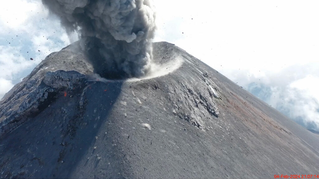
In another case, we landed a pair of Gems on the ground near a frequently exploding crater at Fuego volcano in Guatemala using a drone (see video below). We later retrieved one of the sensors from high on the volcano’s flanks. Another was lost because high winds initially posed too great a risk to fly the drone back for it. Then the following day after the wind subsided, we could not locate the stranded Gem, which was probably a casualty of a nighttime explosion.
Drone footage and infrasound recordings were collected during an explosion of Fuego volcano on 4 February 2024. Pa = pascals. Credit: video: Jerry C. Mock; animation and infrasound: Jeffrey B. Johnson
Our group at BSU also has nascent interest in using Gems to study fire in natural environments. Wildfires produce infrasound from a spatially extensive source region corresponding to actively burning areas. Because of the source complexity and the fact that fire infrasound is low amplitude and tremor-like [Johnson et al., 2025], enhancing signal-to-noise ratios in recorded infrasound is critical. This enhancement is enabled by using large-N monitoring networks, making infrasound wildfire surveillance a promising area of investigation.
Low-cost, rapid infrasound deployments could one day be used as an effective operational tool.
Toward this objective, our group installed 76 sensors ahead of a prescribed burn in Reynolds Creek, Idaho, in October 2023 to begin developing infrasound as a tool for monitoring and mapping wildfire. We have also deployed Gems for infrasound studies of naturally occurring wildfires, such as the Emigrant wildfire in Oregon in August and September 2025 (Figure 3). During that active wildfire response, a team safely and quickly installed tens of sensors within a matter of hours in an area facing dynamic hazards from the rapidly expanding fire, which eventually covered 33,000 acres (about 13,354 hectares). Luckily, no instruments were lost, and the data have shown the potential to track a wildfire as it advances.
Preliminary results suggest that low-cost, rapid infrasound deployments could one day be used as an effective operational tool. For example, in firefighting responses, infrasound might complement intermittent aerial observations, from aircraft or drones, because it provides a continuous record of fire activity. Infrasound surveillance might also be able to “hear” combustion sources within a burn area that is obscured to optical sensing because of clouds or nightfall.
Fig. 3. (a) The spread and severity of the 2025 Emigrant Fire in Oregon, as calculated from prefire (21 August) and postfire (18 October) Sentinel-2 satellite images, are shown. Inset maps show the distribution of 37 Gem sensors rapidly deployed in three arrays. (b) Smoke from the fire rises from the landscape on 31 August during deployment of the sensors. (c) Following the fire, one sensor that had been melted by the fire was recovered with its data card still intact (red circle). dNBR = differenced normalized burn ratio. Click image for larger version. Credit: (a) and (b): Madeline A. Hunt; (c): Jacob F. Anderson
The Evolution of Low-Cost Sensors
Five years ago, the single-sensor Gem was a cutting-edge infrasound logging solution. While it remains a powerful and economical tool for large-N arrays and for sensing in hostile environments, it is evolving.
Boise State University researchers (left to right) Madeline Hunt, Owen Walsh, Jerry Mock, and Jacob Anderson prepare to deploy Gem sensors in Idaho’s Sawtooth Mountains in January 2024. Credit: Jeffrey B. Johnson
We have now developed the Gem into an even more versatile version called the Aspen, which can log four independent sensors at a sample rate of 200 hertz, double that of the Gem. The Aspen retains the small size, low weight, low power consumption, and low cost of the Gem, but with the capability to record higher-resolution 24-bit, time-synchronized data from a triaxial seismic sensor and an infrasound transducer.
Recording synchronous seismoinfrasonic data on the same logging platform offers the advantage of sensing both ground shaking and infrasonic oscillations. The ability to measure waves propagating in the ground and in the air simultaneously could facilitate work in the growing field of environmental seismology, which focuses on geophysical sources at Earth’s surface like debris flows and volcanoes.
Although we have focused on seismoacoustic geophysical measurements in our work, the concept of gathering data with low-cost instrumentation in harm’s way or from coordinated arrays of numerous sensors holds promise across Earth and environmental sciences. Such approaches could be used, for example, with tiltmeters (which measure slope changes), gravity meters, or near-infrared thermometers (e.g., optical pyrometers), all of which would offer additional data streams complementing seismoacoustic observations in geophysical studies of volcanoes.
With the diversity of emerging uses, it’s clear that large-N sensing—infeasible or cost prohibitive in many cases until recently—could transform how we measure many facets of Earth, helping to reveal the inner workings of volatile volcanoes, twisting tornadoes, and more.
Acknowledgments
More information about low-cost infrasound sensing solutions can be found at https://sites.google.com/boisestate.edu/infravolc/home. Development of the Gem infrasound logging platform was supported by a grant from the National Science Foundation (EAR-2122188).
References
Anderson, J. F., et al. (2018), The Gem infrasound logger and custom‐built instrumentation, Seismol. Res. Lett., 89(1), 153–164, https://doi.org/10.1785/0220170067.
Anderson, J. F., et al. (2023), Remotely imaging seismic ground shaking via large-N infrasound beamforming, Commun. Earth Environ., 4(1), 399, https://doi.org/10.1038/s43247-023-01058-z.
Bosa, A. R., et al. (2024), Dynamics of rain-triggered lahars and destructive power inferred from seismo-acoustic arrays and time-lapse camera correlation at Volcán de Fuego, Guatemala, Nat. Hazards, 121, 3,431–3,472, https://doi.org/10.1007/s11069-024-06926-1.
Brissaud, Q., et al. (2021), The first detection of an earthquake from a balloon using its acoustic signature, Geophys. Res. Lett., 48, e2021GL093013, https://doi.org/10.1029/2021GL093013.
Johnson, J. B., et al. (2012), Probing local wind and temperature structure using infrasound from Volcan Villarrica (Chile), J. Geophys. Res., 117, D17107, https://doi.org/10.1029/2012JD017694.
Johnson, J. B., et al. (2018), Forecasting the eruption of an open-vent volcano using resonant infrasound tones, Geophys. Res. Lett., 45, 2,213–2,220, https://doi.org/10.1002/2017GL076506.
Johnson, J. B., et al. (2020), Mapping the sources of proximal earthquake infrasound, Geophys. Res. Lett., 47, e2020GL091421 , https://doi.org/10.1029/2020GL091421.
Rosenblatt, B. B., et al. (2022), Controls on the frequency content of near-source infrasound at open-vent volcanoes: A case study from Volcán Villarrica, Chile, Bull. Volcanol., 84(12), 103, https://doi.org/10.1007/s00445-022-01607-y.
Scamfer, L. T., and J. F. Anderson (2023), Exploring background noise with a large‐N infrasound array: Waterfalls, thunderstorms, and earthquakes, Geophys. Res. Lett., 50, e2023GL104635, https://doi.org/10.1029/2023GL104635.
Slad, G., and B. Merchant (2021), Evaluation of Low Cost Infrasound Sensor Packages, Sandia Rep. SAND2021-13632, Sandia Natl. Lab., Albuquerque, N.M., https://doi.org/10.2172/1829264.
Tatum, T., J. F. Anderson, and T. J. Ronan (2023), Whitewater sound dependence on discharge and wave configuration at an adjustable wave feature, Water Resour. Res., 59, e2023WR034554, https://doi.org/10.1029/2023WR034554.
Author Information
Jeffrey B. Johnson (jeffreybjohnson@boisestate.edu), Jacob F. Anderson, Madeline A. Hunt, Owen A. Walsh, and Jerry C. Mock, Department of Geosciences, Boise State University, Idaho
Citation: Johnson, J. B., J. F. Anderson, M. A. Hunt, O. A. Walsh, and J. C. Mock (2026), Sensing the sounds from Earth’s hazardous environments, Eos, 107, https://doi.org/10.1029/2026EO260142. Published on 8 May 2026.
Source: Journal of Geophysical Research: Solid Earth
Magnetic rocks with iron oxide concentrations act as natural chroniclers of Earth’s past continental movements. Using small samples of rocks, scientists can isolate magnetic grains that were frozen in orientation as the rock solidified. The magnetization of these grains acts as a miniature compass needle, pointing toward ancient magnetic poles. This same principle applies to extraterrestrial samples, such as meteorites and lunar rocks, whi
Magnetic rocks with iron oxide concentrations act as natural chroniclers of Earth’s past continental movements. Using small samples of rocks, scientists can isolate magnetic grains that were frozen in orientation as the rock solidified. The magnetization of these grains acts as a miniature compass needle, pointing toward ancient magnetic poles. This same principle applies to extraterrestrial samples, such as meteorites and lunar rocks, which preserve evidence of the early solar nebula’s evolution.
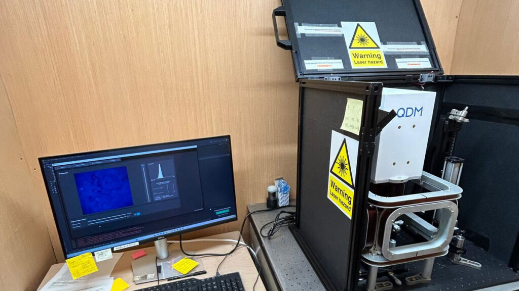
However, traditional bottle cap–sized bulk samples often contain a mixture of reliable and unreliable magnetic signals, resulting in complex data that hamper interpretation. To improve accuracy, researchers have turned to magnetic microscopy. This technique maps magnetic fields at submillimeter to submicrometer scales in thinly sliced rock sections using advanced tools like a quantum diamond microscope (QDM) or a cryogenic superconducting quantum interference device microscope. By creating high-resolution maps of individual magnetic particles, scientists can reconstruct ancient fields with much higher precision while filtering out muddy signals from unstable grains.
Despite its potential, magnetic microscopy is an emerging field with its own set of uncertainties. To help constrain measurement data, Bellon et al. combined QDM observations with computer modeling to analyze how a magnetic particle’s stray field—the magnetic flux that leaks into the surrounding space—decays as it moves away from the source. They specifically investigated how a particle’s internal magnetic structure and external measurement noise affect the accuracy of these reconstructions.
The study found that in iron oxides, the smallest and most magnetically stable particles produce signals that are strong at the source but fade rapidly with distance. In contrast, larger particles produce signals that remain detectable farther away. This creates a challenge: The most stable grains for long-term geological data (the smallest ones) are the hardest to detect if the sensor is not perfectly positioned or if sensor interference is present.
By quantifying measurement error, the authors provide a road map for the field of micropaleomagnetism. Their findings could allow researchers to better account for uncertainty, leading to more robust reconstructions of Earth’s magnetic history and a deeper understanding of planetary evolution. (Journal of Geophysical Research: Solid Earth, https://doi.org/10.1029/2025JB033133, 2026)
—Aaron Sidder, Science Writer
Citation: Sidder, A. (2026), Navigating the past with ancient stone compass needles, Eos, 107, https://doi.org/10.1029/2026EO260122. Published on 16 April 2026.
Research & Developments is a blog for brief updates that provide context for the flurry of news that impacts science and scientists today.
In the contiguous United States, crop irrigation, municipal water supplies, and thermoelectric power generation use more than 224 billion gallons of fresh water every day. Conducting water research or making decisions about water use, until now, often required referencing datasets across various agencies. The U.S. Geological Survey (USGS) National
Research & Developments is a blog for brief updates that provide context for the flurry of news that impacts science and scientists today.
In the contiguous United States, crop irrigation, municipal water supplies, and thermoelectric power generation use more than 224 billion gallons of fresh water every day. Conducting water research or making decisions about water use, until now, often required referencing datasets across various agencies. The U.S. Geological Survey (USGS) National Water Availability Assessment Data Companion (NWDC), announced this week, aims to streamline this process. In part, the tool is designed to help decisionmakers better understand the balance between how high demand and limited supply affect water availability in their communities.
“While the United States has abundant water nationally, regional imbalances between supply and demand may create water challenges affecting millions of Americans,” said lead scientist Shirley Leung in a USGSpress release. “What once required significant resources and time can now be done in minutes, giving communities of all sizes the same foundation for water planning.”
The lower 48 states are home to about 80,000 sub-watersheds, from those in the arid southwest to the Great Lakes Basin, where about 84% of North America’s surface fresh water is located. According to the USGS, the NWDC is the first tool that integrates information about water availability in individual watersheds at a national scale.
The tool is designed to complement Water Data for the Nation (WDFN), another USGS product that consolidates observational data from the agency’s thousands of local monitoring stations gathering data on streams, lakes, reservoirs, precipitation, water quality, and groundwater. The new tool uses modeling to fill in spatial and temporal gaps between the observations made at these stations.
Water managers, researchers, agricultural experts, and others can use the NWDC to compare watershed conditions, identify seasonal patterns in water use, or to create data visualizations of statewide water use, for example. Though the tool currently covers only the contiguous United States, it will soon be extended to Alaska, Hawaii, and Puerto Rico, according to the USGS.
David Tarboton, a professor of civil engineering at the Utah Water Research Laboratory, said he was “intrigued” by the new tool, and is interested in examining the data its model produces.
While Tarboton was disappointed that the tool’s most recent available data are from 2020, “having a sort of integrated, wall-to-wall dataset that’s consistently produced is very valuable,” he said. He works, in part, in the areas of hydroinformatics and data sharing, and noted that the modern methods the agency is using to share the data could be useful in developing automated tools.
These updates are made possible through information from the scientific community. Do you have a story about science or scientists? Send us a tip at eos@agu.org.
Months after wildfires eliminate vegetation that holds hillside sediment together, debris flows—destructive landslides that carry bulky material down once-stable slopes—can devastate infrastructure, taking out roads and buildings in their wake.
Though the U.S. Geological Survey (USGS) creates hazard predictions used to warn communities of the risk of these postfire debris flows, those predictions haven’t fully considered how recovering vegetation reduces risk over time—until now.
A new study published in Geosphere presents a new way to calculate postfire debris flow risk that takes vegetation recovery into account. The USGS will begin using the new method this wildfire season to create more accurate maps of debris flow hazard in the years after a fire.
“I’m so appreciative that the focus on how the debris flow hazard changes over time after fire is being addressed,” said Nancy Calhoun, a geologist and postwildfire debris flow program manager at the Washington Geological Survey who was not involved in the new study. Calhoun said she relies on the USGS hazard assessments for virtually everything her job requires.
“We’re glad to have a way that we can help our partners moderate those situations where the hazard has decreased,” said Andrew Graber, a geologist at the USGS Landslide Hazards Program and lead author of the new study.
Assessing Hazard, Again
After a wildfire, the USGS creates hazard maps that incorporate information about soil type, steepness, and burn severity (how much vegetation has been lost) to show where the risk of a debris flow may be elevated.
Then, the agency distributes this guidance to the National Weather Service, which uses it to set rainfall thresholds: levels of rainfall at which a debris flow becomes likely. State, county, and city agencies use those rainfall thresholds to issue warnings or take action when rainfall is imminent, for example, by closing highways or triggering evacuations.
“That left us with some uncertainty when we started to get further away in time from the fire.”
The methods used to create the USGS maps, however, historically relied on a snapshot of the burned area taken just after the fire, and the maps weren’t updated to reflect conditions as vegetation grew back and began holding soil in place again.
That led to situations where public safety decisions were made on the basis of outdated maps and rainfall thresholds. For example, concern over debris flows after the 2020 Grizzly Creek Fire in Colorado led to several closures of Interstate 70 in 2022, but the debris flows never happened.
“What [the original assessments] didn’t capture is how the vegetation came back,” Graber said. “That left us with some uncertainty when we started to get further away in time from the fire.”
Intense rainfall in July 2025 triggered a debris flow near Dayton, Wyo., in the 2024 Elk Fire burn area. Credit: USGS, Public Domain
To test an improved method for these hazard assessments, Graber and the research team incorporated satellite imagery of 12 burned areas that showed the degree of vegetation recovery right after the fire, 1 year after the fire, and 2 years after the fire. Then, they tested their new method by comparing its predictions to rainfall and debris flow data from the 12 burned areas.
The updated method better reflected what had actually happened after the fires, reducing the number of unnecessary warnings without missing real-world debris flows.
Risk Recalibration
The USGS plans to begin using their new workflow to create hazard maps for some higher-profile fires during the coming wildfire season.
“It’s a really important question: Are we still worried about this burn scar?”
That’s exciting for Calhoun. As part of her job, she’s in constant contact with emergency managers who periodically ask how worried they should be about debris flows in areas that burned years ago. “It’s a really important question: Are we still worried about this burn scar?” she said.
Right now, Calhoun has no data to point to in the years after a fire to give an updated answer to that question. Using the new method from Graber and the research team, she will.
“Because they’re using satellite [imagery] and repeatable quantitative methods to look at these burn scars over time, we’ll actually be able to say something useful and informed about vegetation recovery,” she said.
Having a deeper understanding of how debris flow risk evolves over time is especially important because debris flows themselves are becoming a greater risk to the public as a result of increasingly intense wildfires and rainstorms. In addition, more accurate assessments can reduce warning fatigue, which occurs when too many false alarms lead to people ignoring or opting out of alerts.
Graber hopes he and the USGS will continue to improve their methods for assessing debris flow hazards by collecting more debris flow data across the country and improving the underlying equation for hazard assessments so that it better reflects the unique conditions of different ecosystems in the United States. USGS researchers also published a new study in March presenting a method to generate maps of where debris flows might travel if they do occur.
“It’s a big year for USGS’s useful postfire products,” Calhoun said.
This news article is included in our ENGAGE resource for educators seeking science news for their classroom lessons. Browse all ENGAGE articles, and share with your fellow educators how you integrated the article into an activity in the comments section below.
Citation: van Deelen, G. (2026), A new approach can better predict debris flow hazards years after fires, Eos, 107, https://doi.org/10.1029/2026EO260160. Published on 19 May 2026.