Research & Developments is a blog for brief updates that provide context for the flurry of news regarding law and policy changes that impact science and scientists today.
The National Science Foundation (NSF) has eliminated its postdoctoral fellowship funding for Earth scientists.
On the NSF website, the opportunity is listed as “archived.” This first came to the attention of Eos this week, although a Redditor had posted about the opportunity being archived as far back as March.
“What do you do when the most powerful people in the country just decide that your field shouldn’t exist anymore?” asked one Earth scientist on Bluesky.
“So, what are we doing now that we’re just not going to have new grants in GEO?” asked another.
According to the last program solicitation, posted in October 2024, the program generally awarded about $2.78 million each year, funding 8 to 10 postdoctoral fellowships. Proposals could be related to any of the disciplines within the scope of NSF’s Division of Earth Sciences (EAR), part of the NSF Directorate for Geosciences (NSF GEO).
The NSF announced an “organizational realignment” in December 2025. As part of the agencywide reorganization, GEO gained new leadership in February 2026. Joydip Kundu, the new NSF GEO Directorate Head, first joined NSF GEO in July 2025 as the agency’s deputy assistance director, coming from the NSF Directorate for Computer and Information Science and Engineering. He previously worked for the White House Office of Management and Budget (under President Obama) and the University of Maryland. Like Kundu, NSF’s new deputy directorate heads also came from within the agency.
When contacted about the archived opportunity, an NSF spokesperson confirmed to Eos that “The EAR postdoc fellowship solicitation has been archived and will not have a competition this fall. NSF regularly evaluates its portfolio of funding opportunities and will continue to explore funding opportunities for early career geoscientists.”
NSF continues to offer fellowship opportunities to postdoctoral researchers in the fields of engineering, entrepreneurial research, mathematics and physical sciences. Fellowships to postdocs in biology are available only if they involve the use of artificial intelligence.
These updates are made possible through information from the scientific community. Do you have a story about how changes in law or policy are affecting scientists or research? Send us a tip at eos@agu.org.
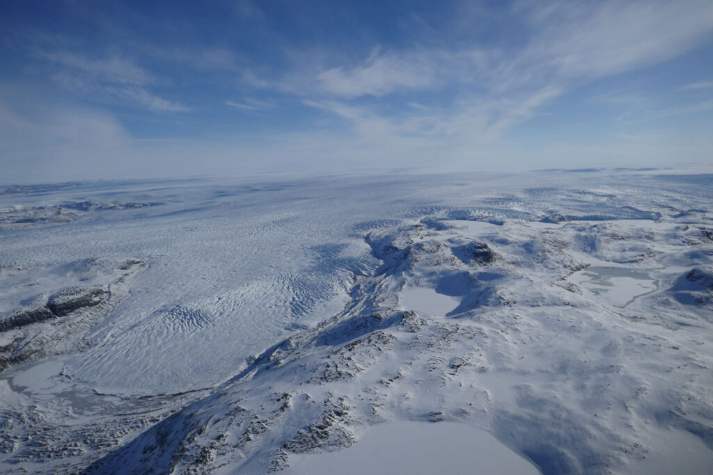
The retreat of glaciers and ice sheets is expected to have widespread impacts on communities around the world because of its effect on sea levels. Already, the global average sea level is more than 10 centimeters higher than it was just 3 decades ago; and the rate of rise is increasing, contributing to increased storm surges and flooding, lost infrastructure and community lands, and more.
Recent reports on the instability of Antarctica’s Thwaites Glacier, for example, have focused attention on how accelerating ice flow can lead to ice sheet collapse and rising sea levels.
Earth’s ice sheets accumulate ice through snowfall and lose mass through a mix of surface ablation, iceberg calving, and melting at their interface with the ocean. Glacial ice flows under its own weight, and the rate at which it flows to coastal areas is a primary control on ice sheet mass loss.
Flow rates depend on how much resistance an ice sheet encounters at its interface with the ground (e.g., whether it is frozen to its substrate) and on its effective viscosity, a measure of how strongly it resists deformation. The viscosity of ice, in turn, varies based on properties including temperature, crystal size and orientation, and impurity content.
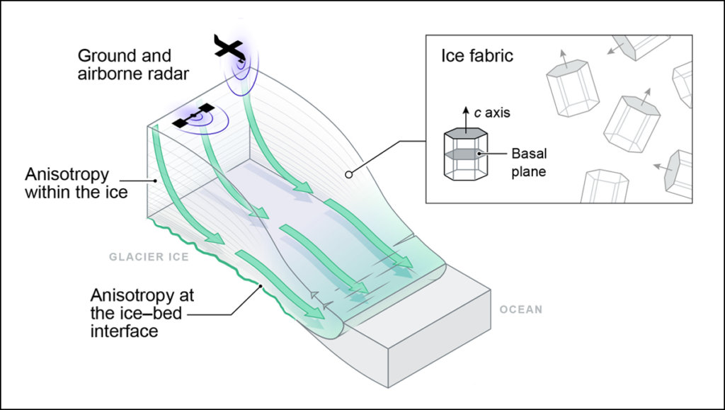
Some properties within and beneath ice sheets that affect how they flow are anisotropic, meaning they vary by direction. For example, roughness in some directions at the ice bed can facilitate ice sliding more effectively than roughness in other directions, similar to the way a properly oriented corrugated metal roof allows snow to slide off. Several forms of anisotropy within ice also affect how ice flows from land to ocean (Figure 1).
Fig. 1. Anisotropy in glaciers and ice sheets has various sources, including from ice fabric and other properties within the ice (englacial) or at the ice-bed interface. Many forms of anisotropy in glacial ice can be measured with radar. Credit: Adapted from Hills et al., 2025, https://doi.org/10.1029/2024RG000842, CC BY 4.0
Measuring anisotropic properties is key to better understanding how quickly changes at the edges of the Greenland and Antarctic ice sheets will lead to sea level rise. Recent advances in ice-penetrating radar technology and in processing radar data are revolutionizing how we observe directionally varying ice sheet properties, paving the way for projections of mass changes that account for previously neglected processes.
Crystal Fabric: Memory and Modulator of Ice Flow
Fabric, the orientation of crystals composing ice, is the best studied and arguably most important of anisotropic ice sheet properties. As ice deforms, for example, by stretching horizontally as it flows toward the coast, its millimeter-scale crystals are reoriented (Figure 1).
Fabric thus contains a memory of past flow. Simultaneously, fabric influences flow because ice crystals are about 3 orders of magnitude easier to shear in some directions than others—similar to how stacked playing cards slide easily against each other when held along their edges but resist motion when pinched top to bottom.
Over the past 20 years, radar polarimetry has matured into a quicker and easier alternative means for inferring fabric.
The potential importance of fabric on large-scale ice flow has long been recognized, but a shortage of observations has made it difficult to quantify and validate its effect in ice sheet models. Until recently, fabric could be measured only directly in ice cores or inferred through seismic soundings. These methods provide highly detailed information about how fabric develops but are expensive, logistically taxing, and provide information only about sparse point locations.
Over the past 20 years, though, radar polarimetry has matured into a quicker and easier alternative means for inferring fabric, enabling observations at the scale of entire glaciers and providing new constraints on how fabric influences ice sheet flow.
How Radar Reveals Fabric
Ice-penetrating radar instruments emit electromagnetic energy as radio frequency waves. These waves reflect off interfaces within and beneath glacial ice, including transitions in ice chemistry and the contact surface between the ice sheet and the ground or water below. The properties of the reflected waves are then measured when they return to the radar. Just as fabric leads to anisotropic ice deformation, it also introduces directional dependence in the measured electrical properties.
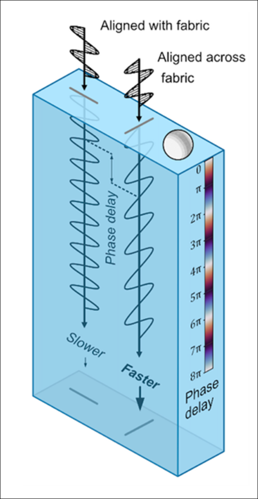
The speed of a radar wave through an ice crystal is approximately 1% faster if the wave is polarized across the crystal’s principal (c) axis rather than aligned with it. Though small, this difference can compound enough that it causes measurable changes in returned radar signals.
In a typical radar survey over anisotropic ice, waves with different polarizations travel at slightly different speeds (Figure 2). The times that return signals arrive back at the receiver thus vary directionally, a difference that can be identified using polarimetric radars that transmit and receive radio waves at multiple orientations.
Fig. 2. Propagation of polarized radio waves through anisotropic ice reveals structural variations with depth because waves aligned across the prevailing ice fabric (represented by the ball, in which darker shading indicates a greater concentration of c axes) travel faster than waves aligned with the fabric. The phase delay increases as the effect of the anisotropy accumulates with depth. Credit: Adapted from Hills et al., 2025, https://doi.org/10.1029/2024RG000842, CC BY 4.0
Fabric’s effect on radar signal travel times accumulates through an ice column, so it is more prominent in thicker ice with stronger horizontal fabric (i.e., the ice crystals are more consistently aligned). In such cases, differences in travel times between polarizations can be measured even by standard radars.
When fabric is weaker or ice is thinner, the offset is smaller and detectable only by systems that can identify the phases of radar returns—that is, the exact positions of the returned waves in their oscillation cycle. Even small wave speed differences from weak fabrics accumulate into measurable phase shifts between polarizations, which can be used to determine the consistency of crystal alignment and the predominant crystal orientation.
Small differences in fabric through an ice column can also change the strength, or amplitude, of returned signals. This amplitude difference offers an independent way to identify fabric orientation and its depth variation.
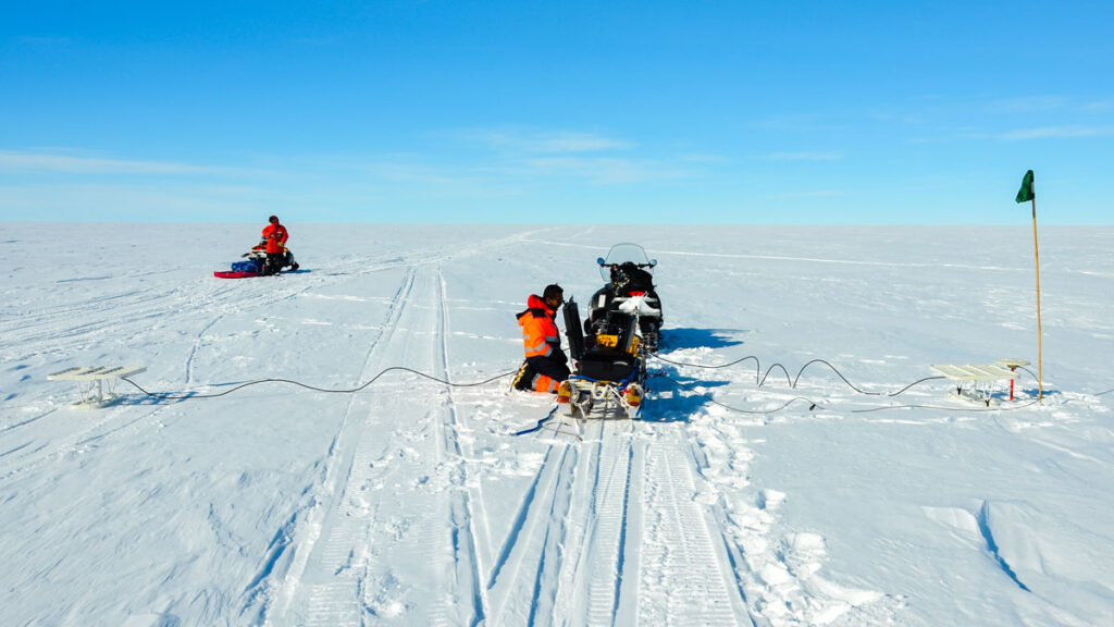
Polarimetric radar has been widely applied in cryospheric science in recent years largely due to the advent of low-cost systems that can measure signal phases. For example, the popular Autonomous phase-sensitive Radio Echo Sounder (ApRES) is a lightweight, ground-based system that can be used to infer ice fabric at single points down to 2 kilometers deep. In the past decade, polarimetric ApRES systems have revealed ice flow histories, including changes in flow directions, of key glaciers over the past few millennia. These measurements offer windows into how ice sheets responded to previous climate variations.
A mobile, quad-polarimetric radar is dragged by snowmobile over the surface of Müller Ice Cap on Axel Heiberg Island in Nunavut, Canada, in May 2023. Credit: David Lilien
The next generation of polarimetric radars go beyond one-point-at-a-time stationary soundings, offering full polarimetry capabilities on moving platforms. These systems may soon allow scientists to map directional ice properties at the scale of entire ice sheets.
Insights into Fast-Flowing Ice Fabric
The growing number of radar studies conducted near sites where ice cores have been collected, which allow fabric to be investigated up close, has provided validation and bolstered confidence that fabric can be inferred accurately from its effects on radar. Researchers now infer fabric from radar in more dynamic areas, such as Thwaites Glacier, Whillans Ice Stream, and the Northeast Greenland Ice Stream (NEGIS), where ice fabrics change over short spatial scales and where drilling ice cores is logistically difficult. Airborne radar surveys are particularly effective in these settings because they can efficiently map fabric variations across large, fast-moving areas.
Observations of strong fabrics in fast-flowing regions suggest that fabric is an important control on ice viscosity, although its implications for ice flow are just beginning to be explored. For example, at Rutford Ice Stream in Antarctica, ApRES data indicate that fabric causes sharp changes in viscosity in different directions with depth, a complexity not captured by current ice flow models.
A combination of airborne and ground-based radar shows that the fabric of the NEGIS varies substantially across the ice stream, which facilitates horizontal shear that allows faster and more cohesive flow in the middle of the ice stream while simultaneously stiffening this ice against along-flow stretching. These viscosity variations may alter how quickly coastal changes, such as increased melt due to climate warming, influence inland ice flow.
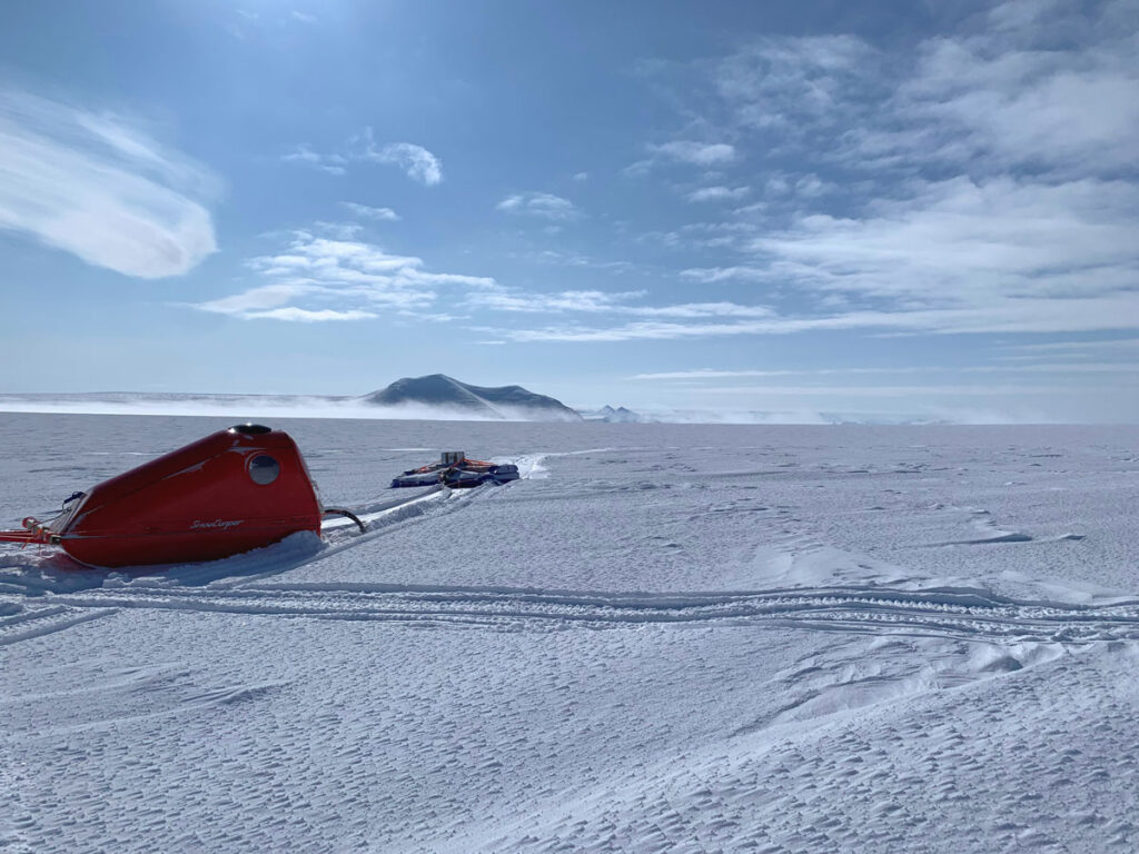
Scientists have studied ice sheet mass balance at glacier-mounted stations along the renowned “K-transect” near Kangerlussuaq in southwestern Greenland since the early 1990s. This image shows a view up the transect in April 2025. Polarimetric radar offers another tool with which to study ice flow here and at other locations on the ice sheets. Credit: Tamara Gerber
The emerging consensus from radar observations and recent progress in fabric modeling is that ice fabric can soften ice stream shear margins by a factor of 10. In other words, the fabric tends to develop in a way that greatly reduces the ice’s effective viscosity at lateral boundaries between fast-flowing and slower-flowing ice, which enables the ice to deform more easily at the margins. The agreement between observations and process-scale modeling highlights fabric as a major, but largely ignored, control on ice flow that may affect estimates of how ice dynamics will contribute to future sea level rise.
Beyond Fabric
Most polarimetric radar studies so far have focused on fabric, but other ice characteristics can cause directional effects too. For instance, bubbles trapped in ice have dramatically different properties than ice itself. Ice deformation can bring bubbles into alignment, such that they affect radar waves differently in different directions.
Likewise, ice at its melting point can contain liquid water along boundaries between crystals, and if those pockets of water are aligned in one direction, they can also affect radar returns. Each of these properties has important influences on ice flow, but their implications are yet to be explored.
Another source of anisotropy is the bottom boundary of the ice sheet. This interface can be rougher in some directions than others, though the roughness is typically aligned with the prevailing ice flow direction or the direction of meltwater trapped within the ice.
Polarimetric radar can measure directionally dependent properties of ice sheet bases at a finer scale than radar profiling can. Such work is leading to new insights into glacier geomorphology, interactions of ice shelf bottoms with the underlying ocean, and how ice slides over substrate surfaces. Rates and extents of sub-ice-shelf melt and basal sliding are widely recognized as key controls on the future of the ice sheets.
Expanding Horizons: Large-Scale and Planetary Applications
Radar polarimetry has already transformed our understanding of ice fabric, revealing much about how crystal alignment modulates the flow of Earth’s ice sheets and filling critical gaps between the handful of direct measurements from ice cores. As polarimetric techniques mature, their applications are expanding.
Researchers are moving from studying isolated profiles of ice fabric to mapping it across whole basins, a key shift for validating bespoke models of fabric and its effects on flow. These models are also rapidly developing to include additional physical processes (e.g., migration recrystallization) and key simplifications (e.g., reducing directionally varying viscosity to a single number) that allow them to interface more easily with—and be incorporated into—large-scale models used for projecting sea level rise.
Techniques pioneered for measuring ice on Earth may also prove useful elsewhere in the solar system.
Techniques pioneered for measuring ice on Earth may also prove useful elsewhere in the solar system. Orbital radar sounders have already probed Mars’s ice masses, and the icy shell of Jupiter’s moon Europa will soon be surveyed by single-polarization radars aboard NASA’s Europa Clipper and the European Space Agency’s Jupiter Icy Moons Explorer (JUICE). These radars might be useful for polarimetry at some locations on Europa, which could reveal past and present motion of ice features and answer fundamental questions about the moon. Whether Europa’s shell flows, for example, may be key to whether its subsurface ocean can harbor life.
As polarimetric radar systems become routine tools for glaciologists and as similar instruments begin operating on spacecraft exploring icy worlds, a technique once limited to a few isolated core sites on Earth could be poised to transform our understanding of ice across the solar system.
Author Information
David Lilien (dlilien@iu.edu), Indiana University Bloomington; T. J. Young, University of St Andrews, Fife, Scotland; Benjamin Hills, Colorado School of Mines, Golden; Tamara Gerber, Université de Lausanne, Lausanne, Switzerland; and Matthew Siegfried, Colorado School of Mines, Golden
Citation: Lilien, D., T. J. Young, B. Hills, T. Gerber, and M. Siegfried (2026), New directions in mapping ice sheet fabrics and flow, Eos, 107, https://doi.org/10.1029/2026EO260154. Published on 14 May 2026.
When it comes to thriving at high elevation, diminutive plants are always a safe bet. And low-lying vegetation is in fact colonizing higher and higher reaches as the climate changes, new results reveal. Researchers analyzed more than 2 decades’ worth of satellite data and showed that the vegetation line in the Himalayas is moving upward, in some cases by up to several meters per year. These changes have implications for the hydrology of the region and therefore for water resources for the population centers located downstream, the team reported last month in Ecography.
Mountains and People
“If you’re going to understand climate change across the Himalayas, you can’t just look at one location.”
The Himalayas, with their massive stores of frozen water, are part of a region known as the planet’s “Third Pole.” Nearly a billion people rely on water sourced from this area, but the Himalayas aren’t immune to climate change—shifts in temperature and precipitation patterns are causing glaciers to melt and permafrost to thaw, among other effects. “The Himalayan mountains are experiencing a lot of ecosystem changes,” said Ruolin Leng, an Earth scientist who led this new research while at the University of Exeter in the United Kingdom. She currently works at H2Tab, a wellness company.
And while the macroscopic effects of climate change in mountainous regions—the melting of the aforementioned glaciers, for example—have been readily studied, shifts in vegetation are often overlooked, said Leng. That’s a problem because plant cover affects everything from soil moisture levels to water runoff to the albedo of the planet’s surface, all of which have consequences for how water moves through the larger system, she said. “It’s a very important factor in the hydrological system.”
Leng and her colleagues focused on six sites, each roughly 40,000 square kilometers in size, in Bhutan, Nepal, and politically disputed areas farther west. Altogether the locales spanned roughly 15° in longitude (about the width of a U.S. time zone). The choice to analyze several locations along an east-west gradient was deliberate, said Stephan Harrison, a climate scientist also at the University of Exeter and a member of the research team. “The western Himalayas are very different from the eastern Himalayas in terms of climate. If you’re going to understand climate change across the Himalayas, you can’t just look at one location.”
Spotting Vegetation from Space
For each of those sites, the researchers mined satellite observations collected from 1999 to 2022 by the NASA/U.S. Geological Survey Landsat program. The researchers focused on visible and near-infrared observations to calculate a metric known as the normalized difference vegetation index (NDVI). Vegetation tends to reflect relatively little visible light while reflecting much more near-infrared light, and that fact can be exploited to infer the presence of vegetation in remote sensing data, said Karen Anderson, a remote sensing scientist at the Environment and Sustainability Institute at the University of Exeter and a member of the research team.
After masking out pixels too obscured by clouds or snow to correctly analyze, Leng and her colleagues calculated the NDVI for each 30- × 30-meter Landsat pixel within their study regions. The team retained pixels with NDVI levels above a minimum threshold and used those data, combined with topography information, to estimate the maximum elevation that was reliably vegetated each year. All six sites exhibited upward trends in the elevations of their vegetation lines over time, the researchers found. A site in central Nepal straddling the country’s northern border recorded the largest changes: From 1999 to 2022, the elevation of its vegetation line rose from roughly 5,520 meters to 5,670 meters, an increase of just under 7 meters per year on average. The five remaining sites all recorded annual upward shifts ranging from about 1 to 6 meters per year on average.
“Broadly speaking, plants are moving up mountains,” said Anderson. But different regions are responding differently, she added. (And while similar results have been previously noted in the Himalayas, not all plant life everywhere is moving up—recent research has shown that some tree lines are in fact moving downslope.)
A Climatic Culprit?
“People neglect the little plants.”
To investigate the potential drivers behind these changes, the team studied correlations with three climatic parameters: temperature, total precipitation, and snow depth. These data came from the European Centre for Medium-Range Weather Forecasts reanalysis dataset, which has a spatial resolution of roughly 30 kilometers.
Leng and her collaborators found that their site with the fastest-changing vegetation line also recorded the most rapid increase in snow depth over time. These two changes might therefore be linked, but more work is needed, Anderson admitted. “We haven’t addressed the causal link here. We’ve simply looked for patterns.”
There’s also a significant mismatch in the spatial resolution of the team’s meteorological data and their Landsat data, said Trevor Keenan, an ecosystem scientist at the University of California, Berkeley not involved in the research. Such a discrepancy can be particularly problematic in complex landscapes like mountain ranges because the coarse meteorological data might not be capturing the true microclimates that are bound to persist in such places, he said. “With heterogenous terrain and large elevational gradients, you really need that microclimate information.”
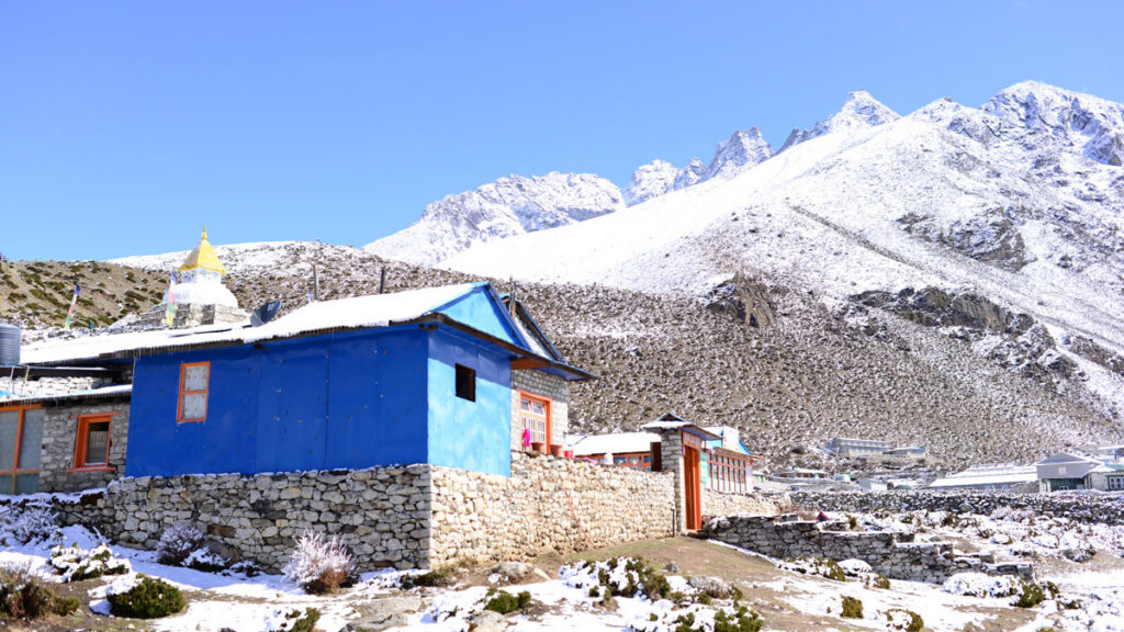
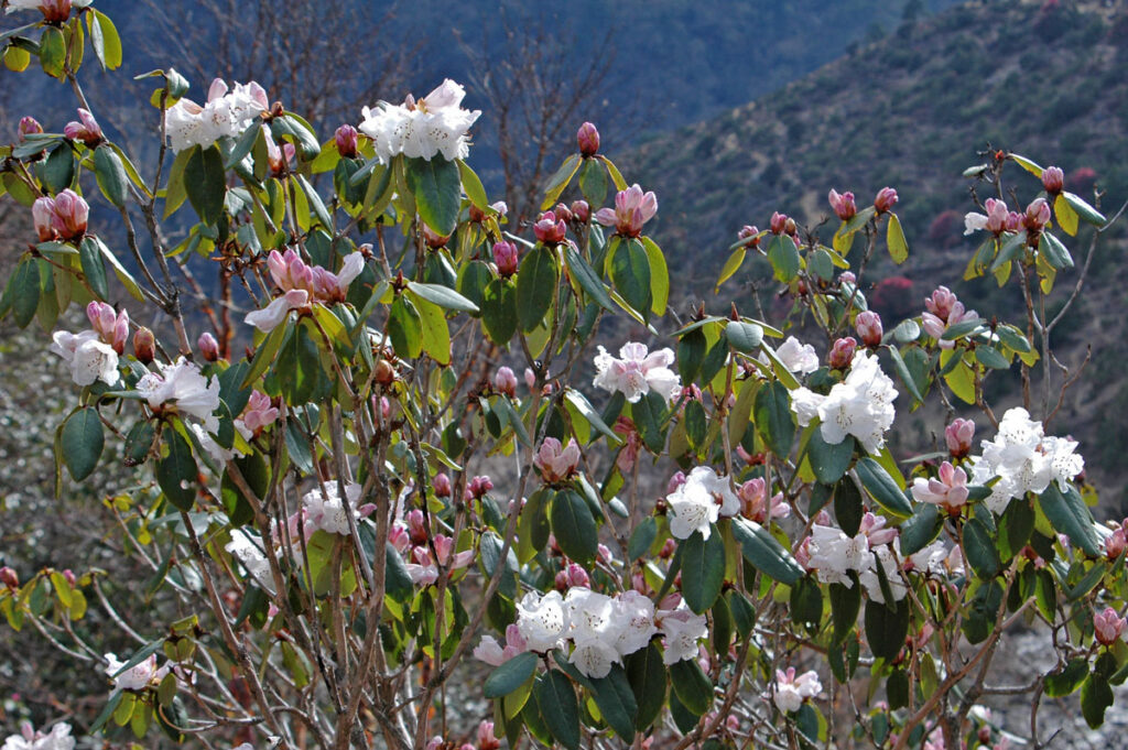
Sagarmatha National Park in Nepal, home to Mount Everest, is also host to rhododendron forests like this one. Credit: Peter Prokosch, CC BY-NC-SA 2.0
Anderson knows the geographical complexity of the Himalayas firsthand—in 2017 and 2022, she and other scientists conducted fieldwork in Nepal that informed this research. Those trips were a special opportunity to see plants like dwarf rhododendron thriving in tough conditions, she said. And it was a good lesson in appreciating some of the most diminutive members of the plant kingdom, Anderson added. “People neglect the little plants.”
Often times when we think “scientist,” we picture a white lab coat, a pipette. Or, a marine biologist covered in seaweed samples. A geologist with dusty knees and hands full of rock fragments. Endless blue gloves. What we may not always picture is our favorite professors, colleagues, or even students advocating for science to policy makers.
Federal policy decisions have a direct impact on science funding, research priorities, and the role of science in society.
Federal policy decisions have a direct impact on science funding, research priorities, and the role of science in society, and the AGU community has a critical role to play in those conversations. Each year, AGU’s Science Policy and Government Relations (SPGR) team organizes and hosts Congressional Visit Days to connect Earth and space scientists to their elected officials. As a member of AGU’s scientific publications team, I joined the April 21-22 Days of Action to learn about the bills currently impacting our workforce and research, how to craft messages that both speak to our personal experiences, and to ask our elected officials to advocate with and for us.
As a D.C. native, I grew up in close proximity to the power of science, the alphabet agencies, NOAA, NASA, NIH, and USDA. Institutions where the best and brightest were given the resources and support to learn, record, and disseminate knowledge on behalf of our country. In my current role with AGU as a non-profit publisher, I took to the Hill to share my experiences on the publishing and academic peer-review landscape. My role allows me to see first-hand how budget cuts and shifting attitudes have impacted critical programs at the agencies named above. This Days of Action event brought together 58 participants with one goal: to share personal stories that related to four bills:
KEEP STEM Talent Act (H.R. 2627, S.1233)- strengthens the U.S. scientific workforce by making it easier for skilled international STEM graduates from U.S. universities to stay in the U.S.
Protect America’s Workforce Act (H.R.2550 passed House, S.2837)- seeks to protect the U.S. federal scientific workforce by restoring collective bargaining (union) rights.
Scientific Integrity Act (H.R.1106)- protects the rights of U.S. federal scientists and researchers by safeguarding scientific integrity in federal research and decision-making.
Two participants spoke on their experiences meeting with elected representatives and uniquely captured just how closely the Earth and spaces sciences touch all of our lives.
Sheila Baber, an early career scientist with The University of Maryland, felt compelled to join due to “the uncertain future for myself, my peers, and the American scientific enterprise.” She noted, “It has been especially difficult to witness the deteriorating relationship between scientists, decision makers, and the public. This past year, with its rapidly changing federal landscape, has been a wakeup call to re-engage and remind the public of how science research gives back to the community.”
Ryan Haupt, long-time AGU member and the Executive Director at National Youth Science Academy, with a 10-year track record of geoscience advocacy, emphasized the importance of building relationships with elected officials. “Regardless of party affiliation, I want those staffers to know that when they meet with me or any other AGU member, they will get honest and informed feedback from folks who are truly passionate about our fields,” Ryan told me. “[Experts who can speak to how current bills] impact issues like improved financial support for graduate students, helping international students stay in the US to join the STEM workforce, and protecting funding for federal science agencies and the folks who work for them.”
As a participant myself, I joined the Maryland group to meet with Senator Chris Van Hollen’s office. Van Hollen and I met briefly at the Stand Up for Science March in 2025. His voting track record indicates a long-standing commitment to the scientific community, and he champions bills that support funding federal agencies like NOAA.
(left to right) The Maryland group, McKay Porter, Andrew Inglis, Nour Rawafi, Stephen Jascourt, and Emille Beller met with Senator Chris Van Hollen’s staffer, Leo Confalone. Credit: Beth Bagley, AGU
Finding and discovering the best and the brightest means funding, protecting, and supporting the best and the brightest.
Working in scientific publishing has allowed me to peer behind lab doors, into research vessels sailing through the Arctic, and into the entire ecosystem that is peer-reviewed research. A system that relies on incoming eager students, federal grant funding, consortium agreements between the biggest institutional libraries and the biggest publishing houses in the country, scientific integrity, and future, stable career opportunities. Finding and discovering the best and the brightest means funding, protecting, and supporting the best and the brightest.
Open, accessible science builds and supports both public trust and future scientific advancements. As the world widens and we are all met with increased access to studies, content, and news, scientific storytelling and literacy have never been more important for ensuring public trust. Transparency from the lab and from the field to published output allows for data to be discussed, fact-checked, and reused to support future scientific discovery. Days of Action demonstrates that we have a unique role to play in supporting the health, safety, and future of our country. If you feel called to get involved, please see resources available from SPGR.
Ryan reminds us, “There are lots of ways to participate in our democracy… find where you can best serve as a leader…don’t try to do it all, but try to do something.”
Citation: Beller, E. (2026), The impact of advocacy: American Geophysical Union’s Days of Action, Eos, 107, https://doi.org/10.1029/2026EO265020. Published on 14 May 2026.
This article does not represent the opinion of AGU, Eos, or any of its affiliates. It is solely the opinion of the author(s).
New Zealand is a country that is prone to a range of natural hazards. Located on a series of major fault systems, earthquakes cause high levels of loss. The country is also volcanically active, with occasional tragedies. Heavy rainfall brings floods.
In the subsequent years, the EQC has evolved into the Natural Hazards Commission – Toka Tū Ake (NHC), with a purpose “to reduce the impact of natural hazards on people, property, and the community”. Essentially it operates as a financial pool, with home owners paying a levy on top of their insurance to generate the fund. In the event of a loss, the fund pays for the rebuild costs up to a cap (currently NZ$300,000); the remainder is then covered by the property’s insurance. Claims are funded directly from the pool, with reinsurance cover and ultimately a government guarantee in place to ensure that there are sufficient funds.
In reality, NHC does much more than this, acting to manage and settle claims, and to understand the range of hazards to which New Zealand is prone.
In the last few days, a range of media outlets in New Zealand have been reporting new data from NHC about losses from natural hazards in New Zealand. This is the headline from 1News:
“Landslides are New Zealand’s most expensive natural hazard – and new data reveals a sharp rise in damage claims and growing risks to homes, infrastructure and communities.”
In total, since 2021 NHC has received 13,000 landslide claims and has paid out NZ$322 million (US$191 million). New Zealand is seeing an abrupt increase in landslide losses, driven primarily by increasingly frequent high magnitude rainfall events. NHC is urging property owners to undertake preventative maintenance and to be aware of the limitations of EQC cover.
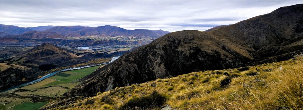
Here be landslides – typical landslide-prone terrain in New Zealand.
In common with many other places, these landslide hazards represent a major challenge to New Zealand. The landscape has many dormant landslides that are being reactivated by these increased rainfall events, and many new failures are also occurring. But, generating reliable risk maps for landslides remains a major challenge. This needs to be a major research focus in the coming years. It will require better understanding of triggering events (rainfall and earthquakes primarily); of the initiation processes within the slope; of runout / debris mobility; and of vulnerability and consequent losses. It is probably true to say that in all of these areas, landslide research lags behind that of earthquakes and floods, primarily because of a lack of long term investment.
In many countries, landslides are not an insured risk for this reason. On its own, this will be a major challenge that must be addressed. For those countries in which landslides are insured, we need quickly to get up to speed.
Research & Developments is a blog for brief updates that provide context for the flurry of news that impacts science and scientists today.
To date, astronomers have confirmed the existence of just under 6,300 exoplanets. New research could more than double that number, adding a potential 10,000 new planets in one fell swoop.
Yes, that’s right. A 1 with 4 zeros.
The T16 project has announced the discovery of 10,091 exoplanet candidates observed by NASA’s Transiting Exoplanet Survey Satellite (TESS). Since 2018, the all-sky survey has been monitoring more than 200,000 nearby stars using the transit method, which detects the faint dip in a star’s light when a planet crosses in front of it. Astronomers typically require 3 dips to be sure that what they’re seeing is actually a planet and not a one-off event such as an asteroid or comet in that distant star system.
The T16 project analyzed the light curves of more than 54 million stars observed during the first year of the TESS mission. The project’s analysis technique allowed it to search for planets around stars up to 16 times fainter than TESS typically searches, drastically increasing the field of discovery.
That’s more than were detected in the entirety of NASA’s Kepler mission and its follow-on K2.
Their pipeline detected 11,554 planet candidates. Of those, 1,052 of those had been detected previously and 411 only had one transit—not enough to confirm a planet.
That leaves 10,091 potential new planets. That’s more than were detected in the entirety of NASA’s Kepler mission and its follow-on K2 and more than double the existing planet candidates from TESS that await confirmation. These discoveries will be published in the Astrophysical Journal Supplement.
All of the new planet candidates orbit their stars quickly, with orbital periods between 12 hours and 27 days. Although most of the stars that TESS observes are smaller and cooler than the Sun, those close orbits likely mean that most of those planets are far too hot to be habitable.
The T16 project team confirmed the planet-hood of one of their candidates not using the transit method, but a different method that measures the gravitational tug a planet exerts on its host star. That planet, TIC 183374187, is hot and slightly larger than Jupiter.
The remaining 10,090 newly discovered planet candidates require additional verification to determine whether they truly are planets or not. But given the rigor of the team’s analysis and the requirement of at least 3 transits to even make this list, it’s likely that most of the new discoveries are indeed planets.
“Astronomers are a bit conservative when it comes to claims like this, and want to be sure they pass a bunch of tests to make sure everything was done correctly and these planets actually exist,” astronomer Phil Plait wrote in his Bad Astronomy Newsletter. “Having said that, the process the astronomers went through looks legit to me, and I would bet the majority of these new candidates are real. That’s amazing.”
These updates are made possible through information from the scientific community. Do you have a story about science or scientists? Send us a tip at eos@agu.org.
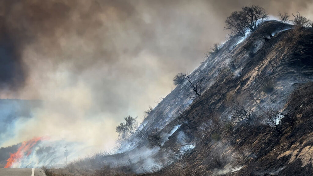
California is no stranger to the hot, dry summer weather that makes wildfires more likely. But wildfire season in the state is now stretching into the heart of winter, when it has historically been protected by cool, wet weather. In January 2025, Southern California experienced some of the deadliest and costliest wildfires in the state’s history.
Now, a new study published in Nature Communications shows that the climatic changes that increase the risk of these winter wildfires could be driven by low autumn snow levels thousands of miles away, in western Eurasia. The authors said that tracking snowfall in Eurasia could help forecast winters in California that will have higher chances of wildfires.
The researchers were motivated by the catastrophic 2025 wildfires to search for climate drivers of winter wildfire conditions in California. First, they looked for correlations between winter wildfires and ocean temperatures, especially La Niña events that are associated with drier-than-average conditions in California. They also examined variability in sea ice, which can affect global weather patterns. But they saw only weak connections.
Compared to oceans and sea ice, the influence of snow cover on global weather patterns is less studied, said Shineng Hu, a climate scientist at Duke University and lead author of the paper. But another climate researcher in Hu’s lab had previously studied the connection between snow cover and weather patterns and suggested the team look for connections between snow and fires. That’s when they found significant correlations between the winter wildfires in California and low snow cover in western Eurasia.
“When I saw the result, I was suspicious,” Hu said, “because we all know that correlation doesn’t mean causality.” But they ran hundreds of climate model simulations reducing snow cover in Eurasia and saw an increased probability of winter fires in California. “At that point, we were pretty much convinced that there could be something interesting happening over there,” Hu said.
Propagating Pressure
“I’m glad to see this group saying snow can do something similar to what ocean temperature anomalies can do.”
The scientists determined that this intercontinental link starts because the land absorbs more energy when snow cover is low, disturbing the atmosphere above it. This disturbance, like a stone thrown into water, generates large waves of air called Rossby waves that travel eastward along the jet stream across the Pacific Ocean. The Rossby waves drive the formation of a high-pressure zone that creates the hot, dry, windy conditions conducive to wildfires.
“I’m glad to see this group saying snow can do something similar to what ocean temperature anomalies can do,” said Judah Cohen, a climatologist at the Massachusetts Institute of Technology who was not involved in the study but has also studied the links between snow in North America and Eurasia. “I’ve been surprised by how important this mechanism is for U.S. weather in the winter and how little there is about it in the literature.”
“This is just one missing gap that people didn’t even realize. We want to add that to the table.”
But Cohen suggested the study tells only part of the story. In North America, dry winters in the west are paired with wet, cold winters in the east. The same is true in Eurasia, and according to Cohen’s past research, when snow levels are low in western Eurasia but high in eastern Eurasia, a temperature and pressure gradient is created across the continent. The energy released as the atmosphere works to equalize that pressure drives the Rossby waves. Cohen said the disparity between snow levels in eastern and western Eurasia would likely strengthen the Rossby waves and then the warming in California. “If all of Eurasia [had] below normal [snow levels], I don’t think you could easily excite this wave energy that propagates across the hemisphere.” He also stressed that Rossby waves don’t just travel eastward. They also travel upward into the stratosphere, where they bounce back down over North America and intensify the high pressure over the western United States.
Both Cohen and the study authors insisted that many other factors influence whether wildfires ignite in winter. “This is just one missing gap that people didn’t even realize. We want to add that to the table,” said Hu. But monitoring snow levels in Eurasia could offer signs of bad wildfire winters to come. The January 2025 Southern California fires were preceded by low snow levels in November and December in Eurasia, Hu said. “So there’s a 1‑month lag, which gives us some hope that we can use that for prediction.”
Citation: Chapman, A. (2026), Low snow in Eurasia linked to wildfires in California, Eos, 107, https://doi.org/10.1029/2026EO260138. Published on 13 May 2026.
For decades, regulators built their ocean monitoring programs mainly around pesticides and pharmaceuticals, treating them as the primary chemical threat to ecological and human health.
That assumption left a much larger category of compounds largely unexamined: the industrial chemicals embedded in packaging, furniture, and everyday personal care products. Those chemicals, it turns out, have been spreading widely. And they’re now showing up even in the places some might consider pristine, such as coral reefs in the Caribbean.
These compounds are biologically active, some interfere with microbial metabolism, and according to a sweeping meta-analysis published in Nature Geoscience, they may be altering how the ocean cycles carbon, one of our planet’s most critical biogeochemical processes.
“Beyond the usual [pesticides and pharmaceuticals], what really surprised us was that everyday industrial chemicals are showing up at even higher levels and not just in coastal or polluted areas, but pretty much everywhere,” said Daniel Petras, a biochemist at the University of California, Riverside.
Led by Petras and Jarmo-Charles Kalinski, a postdoctoral fellow at the Rhodes University Biotechnology Innovation Centre, the study reanalyzed 21 publicly available datasets comprising seawater samples collected over more than a decade across the Pacific, Indian, and North Atlantic Oceans, including the Baltic and Caribbean Seas.
All groups the researchers examined—industrial pollutants, pharmaceuticals, and pesticides—belong to a class called xenobiotics: human-made organic compounds that are foreign to natural systems. Pesticides and pharmaceuticals were prevalent in coastal samples, as expected, given their well-documented entry through agricultural runoff and wastewater outfalls.
But industrial compounds behaved differently. Polyalkylene glycols used in hydraulic fluids, phthalates from polyvinal chloride (PVC) packaging, organophosphate flame retardants from furniture and electronics, and surfactants from personal care products proved far more widespread across all ecosystem types than either pesticides or pharmaceuticals. “These are chemicals we use all the time,” Petras said, “so they end up spreading widely.”
Glimpsing What Was Always There
To map the ocean’s full chemical landscape, the researchers analyzed more than 2,300 samples from temperate coastal zones, coral reefs, and the open ocean, searching for the presence of xenobiotics and examining the share of dissolved organic matter (DOM), a pool of carbon-containing molecules dissolved in seawater. In total, the team identified 248 known xenobiotic molecules. Their work offers the most comprehensive chemical map of anthropogenic organic pollution in the ocean to date.
Researchers used nontargeted mass spectrometry paired with scalable computational tools. Unlike conventional targeted analysis, which tests only for a predefined list of known hazardous molecules, this open-ended approach can detect thousands of chemicals simultaneously, even at low concentrations. The team then applied molecular networking, a computational technique that enables the identification of not only known substances but also their “families” or derivatives.
Coral Reefs as Far-Flung Hot Spots
“Our traditional idea of ‘pristine’ needs a serious rethink, as anthropogenic potential sources are now present nearly everywhere.”
For Petras, it was surprising to find these compounds in coral reefs like those in French Polynesia, which are typically viewed as perfect, “postcard-style” paradises. Yet closer examination reveals that these areas are, indeed, rarely isolated. Agriculture, urban runoff, hotel infrastructure, and cruise ship traffic all contribute pollutants. Remnants of human activity, such as sunscreen, wastewater, and boat fluids, are concentrated near reefs.
“We specifically detected plasticizers and flame retardants even in these remote areas,” Petras said. “This suggests that our traditional idea of ‘pristine’ needs a serious rethink, as anthropogenic potential sources are now present nearly everywhere.”
Anastazia T. Banaszak, a researcher at the Reef Systems Unit of the Universidad Nacional Autónoma de México who was not involved in the study, stressed the broader implications for reef conservation: “Inadequately treated urban wastewater discharges pose a risk to coral reefs and the success of restoration projects,” she said. Such discharges raise nutrient levels, fueling macroalgal blooms that grow faster than corals and compete with them for space. This pressure on ecosystems is intensifying as climate change shifts the baseline against which restoration outcomes are measured, Banaszak noted.
Carbon…and Microbes?
Beyond reefs, these synthetic compounds could be affecting the ocean’s carbon cycle. DOM is one of Earth’s largest carbon reservoirs, comparable in size to all the carbon dioxide (CO2) in the atmosphere. Marine microbes transform it from readily degradable forms into biologically resistant ones; refractory DOM that escapes microbial consumption accumulates in the ocean and acts as an important climate regulator.
But with industrial compounds representing up to 63% of DOM in some estuarine samples (with a global estimate of 10%), the microbial loop is, perhaps, facing chemical conditions it did not evolve to handle. This shift means the efficiency of the ocean’s carbon pump, the mechanism that pulls CO2 from the atmosphere, could be compromised in ways that are not yet understood.
“The data suggest they are present at substantial levels,” Petras said. “Enough that they should be considered in models of carbon cycling.”
Handling the Invisible
Finding xenobiotics is only the first step, the authors say. They laid out several suggestions for next steps. For instance, governments should mandate open-ended approaches as a standard monitoring tool, not just targeted testing of preselected chemicals. Oceanographic data also should be publicly available and standardized, following FAIR (findable, accessible, interoperable, reusable) principles.
“There’s already a strong track record of building long-term datasets for things like trace metals and nutrients. I hope that nontargeted analysis could become part of such long-term efforts,” Petras concluded. “We’ve been quite active in establishing these tools for the community.”
Citation: Mastache-Maldonado, M. (2026), Have we been focusing on the wrong ocean pollutants? This study maps what we’ve been missing, Eos, 107, https://doi.org/10.1029/2026EO260151. Published on 13 May 2026.
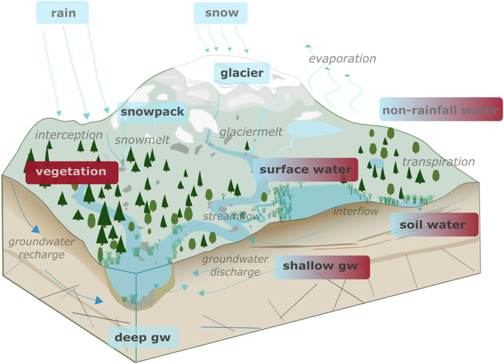
Ensuring the sustainability of water resources and ecosystems in a changing world requires a thorough understanding of how water moves through Earth’s Critical Zone, a dynamic interface where air, water, soil, plants, and rocks interact. Researchers can track and model this movement of water using naturally occurring markers or “tracers.”
A recent article in Reviews of Geophysics explores the latest advancements in tracer-aided mixing models and how they can help us to better understand the Critical Zone. Here, we asked the authors to give an overview of the Critical Zone, how tracer-aided mixing modeling works, and future directions for research.
What is the Critical Zone (CZ)?
The Critical Zone is Earth’s “living skin”—the dynamic layer where the atmosphere, hydrosphere, biosphere, and lithosphere interact. It stretches from the top of the vegetation canopy and, in cold regions, from the surface of snowpacks and glaciers, down through soils and into the deeper aquifers. It encompasses lakes, streams, and wetlands at the surface, and extends beyond the soil layer to underlying groundwater aquifers. It is where rainfall, snowmelt and glacier melt become soil moisture, where plants take up water and return it to the atmosphere, where aquifers get recharged, and where streamflow is generated. In short, the Critical Zone is where most processes that sustain terrestrial life and freshwater resources unfold.
Why is it important to understand how water moves through the Critical Zone?
Virtually every freshwater resource we rely on (e.g., drinking water, irrigation) passes through the Critical Zone.
Virtually every freshwater resource we rely on (e.g., drinking water, irrigation) passes through the Critical Zone at some point. Global warming, land-use changes, and intensifying water demand emerging from rapid urbanization and changes in agriculture are reshaping how water is stored and released within the Critical Zone, often in ways we cannot yet predict. Understanding how much water is stored within the Critical Zone, how this water is both recharged from rainfall and snowmelt and eventually discharged into streams, and the timescale of these dynamic processes is essential for protecting ecosystems, safeguarding water supplies, and adapting to a changing climate.
How would you explain a tracer-aided mixing model to a non-specialist?
Imagine mixing a glass of orange juice with a glass of apple juice, and trying afterwards to work out how much of each went into the glass. If the juices had distinctive “fingerprints” (imagine its color, sugar content, or a specific chemical) and these fingerprints primarily changed because of the mixing of these two juices, you can then measure the fingerprint in the final mixture and back-calculate the proportion of its distinct sources.
Tracer-aided mixing models work in a similar way but can track the entire water cycle. Different water sources (e.g., rainfall, snowmelt, glacier melt, soil water, groundwater) can have distinct “fingerprints” in a naturally occurring tracer, such as stable isotopes of water or specific dissolved elements. By measuring these fingerprints in the streamwater or groundwater and in its potential sources for example, hydrologists can estimate how much each source contributed to the streamwater or groundwater.
Conceptual model of the different components of the Critical Zone. “Gw” stands for groundwater. Credit: Popp et al. [2025], Figure 2
What are some of the most significant and exciting recent advances in tracer-aided mixing models?
Classical mixing models relied on demanding assumptions: that all water sources can be identified and sampled, and that their signatures were distinct and constant in time. Much of the recent progress has been about relaxing these assumptions.
Bayesian approaches now estimate full probability distributions and provide a more realistic picture of uncertainty. Methods like Convex Hull End-Member Mixing Analysis (CHEMMA) use machine learning to infer the distinct sources directly from data, while ensemble hydrograph separation exploits tracer fluctuations over time, thereby making un-mixing feasible even when multiple sources have overlapping signatures. Perhaps the most conceptually novel advance is end-member splitting, which flips the question from “where does streamflow come from?” to “where does precipitation go?”
Alongside these modeling advances, there have been immense advances in how tracers are measured. Portable laser and mass spectrometers now enable high-frequency, in-situ tracer measurements which allows us to capture critical hydrological events such as storms and snowmelt in near-real time.
What are stable water isotope tracers and what are their advantages?
Stable water isotopes are naturally occurring non-radioactive atoms of hydrogen and oxygen that make up a water molecule but have slightly different molecular masses. The two stable isotopes widely used in hydrology are 2H (deuterium) and 18O (oxygen-18). Because these isotopes are part of the water molecule itself, they directly travel with the water molecule. Their key advantages are: (1) they are conservative, meaning they do not react chemically as water moves through soils and aquifers, and (2) they carry distinct signatures resulting from climatic variables such as air temperature.
These properties make stable water isotopes the most versatile and widely used tracer in Critical Zone hydrology.
Consequently, in the European Alps, winter precipitation has a different isotopic signature than summer precipitation because winters are cooler than summers. Other hydrological processes such as evaporation and sublimation leave a recognizable fingerprint on the remaining water, thereby allowing us to estimate how much evaporation or sublimation occurred. Stable water isotopes can be measured in essentially every water compartment, from atmospheric vapor and precipitation to snowpack, plant xylem, soil water, streams, and groundwater. Together, these properties make stable water isotopes the most versatile and widely used tracer in Critical Zone hydrology.
What are the current limitations of tracer-aided mixing models?
Despite their power, mixing models still face many constraints. End-member signatures vary in space and time, are sometimes too similar to distinguish, and some sources may be overlooked entirely. Non-conservative tracers such as nitrate or sulfate can react with their environment along their journey, thereby biasing results if these reactions are not explicitly accounted for.
Sampling is another major bottleneck. Capturing the spatial heterogeneity of soils, snowpacks, and groundwater requires a lot of measurements that are often logistically or financially prohibitive, especially in remote regions. Many of the newer, more powerful tracers such as noble gases or stable isotopes of trace elements, can only be analyzed by a handful of specialized laboratories. As a result, global coverage remains highly uneven, with key regions such as the Arctic and the global South still under-sampled.
What are some of the major unsolved questions and where is more research needed?
There are several fronts where more research is needed. Source signatures are not static, and methods that explicitly capture their variability in time are still underdeveloped. Embedding tracers within global Earth System Models would, in theory, enable more accurate assessment of hydrological partitioning e.g., how rainfall, snowmelt, and glacier melt are split between sublimation, evapotranspiration, groundwater, and streamflow. These will directly inform more robust climate projections, but this remains technically demanding.
Expanding data coverage in under-sampled regions is critical, and citizen science and low-cost sensors may help. Machine learning is a promising approach for uncovering non-linear relationships and gap-filling sparse datasets, but requires training data that often do not yet exist. Greater interdisciplinary integration, e.g., combining tracers with remote sensing, ecological indicators, and biogeochemical data, could yield a more holistic view of the Critical Zone. Finally, the field would benefit from shared protocols and open data practices to enhance progress.
Editor’s Note: It is the policy of AGU Publications to invite the authors of articles published in Reviews of Geophysics to write a summary for Eos Editors’ Vox.
Citation: Popp, A. L., and H. Beria (2026), Tracing water’s hidden journey through the Earth’s living skin, Eos, 107, https://doi.org/10.1029/2026EO265019. Published on 13 May 2026.
This article does not represent the opinion of AGU, Eos, or any of its affiliates. It is solely the opinion of the author(s).
Research & Developments is a blog for brief updates that provide context for the flurry of news that impacts science and scientists today.
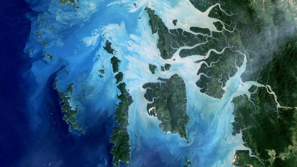
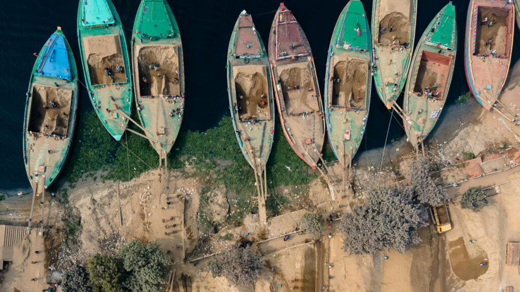
Sand is the most exploited solid natural resource on Earth. It has been integrated into how we build homes, roads, buildings, and bridges as well as how we protect coastal infrastructure from rising seas. Sand underpins nearly every aspect of modern infrastructure and economics, plays crucial roles in supporting ecosystem biodiversity, and literally shores up rivers and coasts.
A new report from the United Nations Environment Programme (UNEP) found that we are using 50 billion metric tons (50 trillion kilograms) of sand per year. As global development and industrialization expand, demand for sand in the building sector is expected to rise 45% by the year 2060, outpacing current efforts to sustainably harvest it. The report’s authors urge countries to establish sand as a strategic national asset and develop policies for sustainable extraction.
“Sand is sometimes referred as the unrecognized hero of development, but its essential role in sustaining the natural services on which we depend is even more overlooked,” Pascal Peduzzi, director of the UNEP Global Resource Information Database Geneva, said in a press release about the report. “Sand is our first line of defence against sea level rise, storm surges, and salination of coastal aquifers—all hazards exacerbated by climate change.”
Sand Wanted: Dead or Alive
Dead sand, or sand that has been extracted from its natural environment, is a key component in building materials like concrete and asphalt. Communities around the world use sand in water filtration systems, providing clean water for drinking and agricultural use. And although a transition to clean energy sources is necessary to curb the effects of climate change, many of those sources also depend on sand: solar panels require glass made from high-purity silica sand, and wind turbines, hydroelectric dams, and nuclear power plants all require concrete.
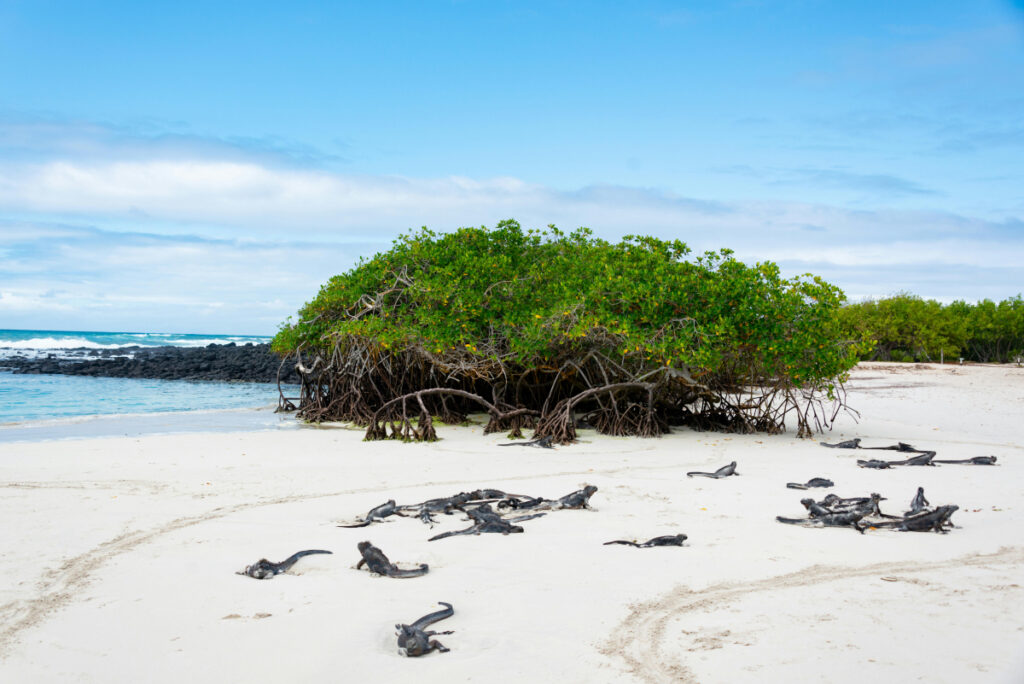
Mangroves, one of the most important coastal trees, can grow in sand. Credit: Diego Parra
Sand also plays a critical role in natural ecosystems. It is home to a wide array of critters from crabs, sharks, and turtles to microorganisms like bacteria and fungi. It supports the growth of corals, mangroves, and seagrasses that in turn support even more marine creatures. It is a key component of healthy soil and aids in surface drainage. It guides river evolution and acts as flood buffer and storm barrier. It also provides local economic benefits via tourism.
These are among the values of sand when it is left alone and unused, called “alive” sand. The UN report notes that these benefits are typically of greater value over time than if sand is dredged and used. But because these benefits are hard to see, they are often overlooked when nations calculate the value of their sand resources.
A Sustainable Sand Future
Despite sand’s importance whether dead or alive, the report notes that few countries have established sand as a strategic national asset or have developed strategies for sustainable extraction. At the current pace, humans are extracting sand from the natural environment at a faster pace than it is being replenished by geologic processes.
What’s more, the UNEP’s Marine Sand Watch tool shows that about half of sand dredging companies are operating within marine protected areas, accounting for about 15% of the volume of dredged sand. This practice, the report notes, is potentially trading in sand’s long-term benefits for short-term gains.
The UN report recommends a few actions to protect the long-term availability of sand as a natural resource, including:
Recognizing sand as strategic national asset, establishing national inventories, and creating long-term regional planning groups that consider sand as an essential resource for resilience;
Establishing circularity and recycling of building materials, especially in areas of conflict and natural disasters;
Strengthening environmental protection practices, and codifying international frameworks to strengthen accountability along the supply chain, including increased transparency about extraction; and
Integrating sand-related biodiversity and social risks into financial decisionmaking and governance.
“Over-reliance on short-term economic metrics risks obscuring, and further impacting, the geological and ecological processes that take centuries to form and may not be restored once critical thresholds are crossed,” the report states. “What is hardest to measure may be precisely what sustains both nature and human societies over the long term. The challenge ahead is not only to manage extraction, but to recognise and balance the full spectrum of sand’s values.”
These updates are made possible through information from the scientific community. Do you have a story about science or scientists? Send us a tip at eos@agu.org.
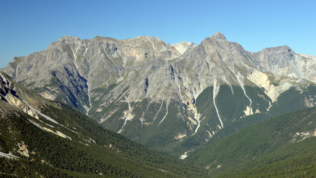
As the climate warms, tree lines are generally understood to move up, because regions that were previously too cold for trees to survive now have higher, more tree friendly temperatures.
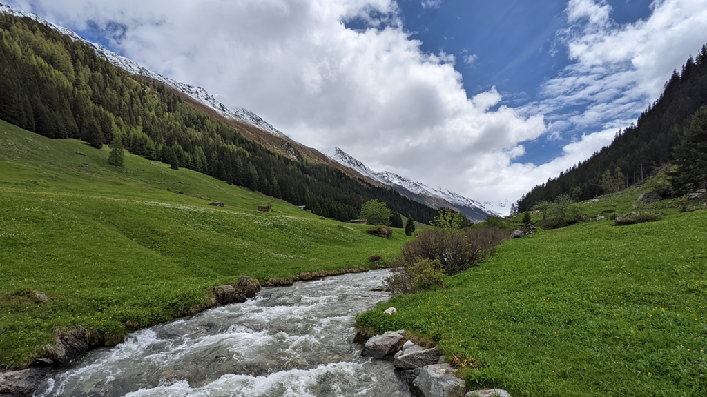
A tree line is clearly visible in the Swiss National Park, in Graubünden, Switzerland. Credit: Sabine Rumpf, University of Basel
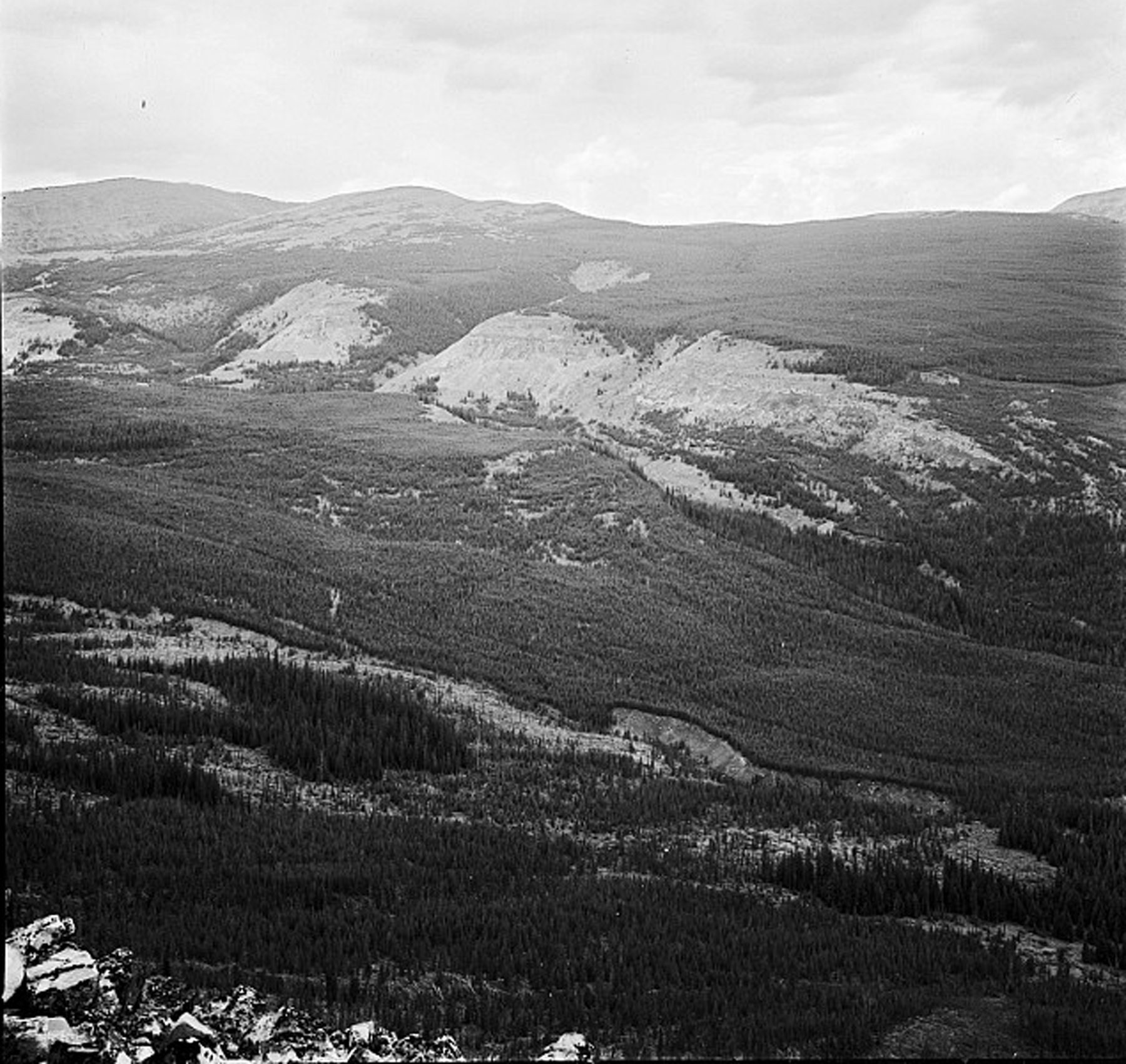
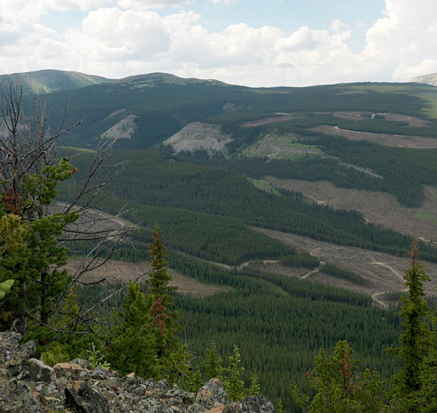
This migration can be seen in these images of Canada’s Waterton Lakes National Park…
Rising tree lines are visible in Canada’s Waterton Lakes National Park, seen here in 1913 (left) and 2007 (right). Credit: Mountain Legacy Project
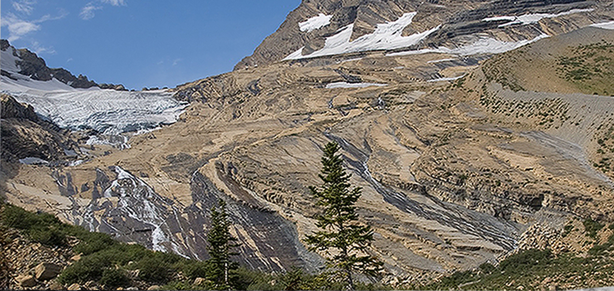
…and of Jackson Glacier in Montana’s Glacier National Park, for example.
Jackson Glacier, in Montana’s Glacier National Park, is seen here in 1912 and 2009. As the climate has warmed, the glacier has receded significantly, and tree lines have risen. Credit: MJ Elrod, U of M Library–9/3/2009, L McKeon, USGS
But new research, published in the International Journal of Applied Earth Observation and Geoinformation, paints a more complicated picture: Between 2000 and 2020, 42% of tree lines shifted up, true. But 25% of them actually moved downhill.
Sabine Rumpf, an ecologist at the University of Basel in Switzerland, said many studies of tree line shifts tend to be concentrated in limited geographic areas. A preponderance are based primarily on data from North America, Europe, and the Himalayas, where researchers are more likely to have funding to head to the field to take measurements themselves.
“But that also means that a large proportion of the surface of our planet is so understudied,” Rumpf said. “And [to remedy] that, remote sensing data [are] really amazing because you can get a truly global picture, even though there’s nobody, or too few people, observing things in the field.”
Tree Lines Aren’t Living up to Their Potential
So the team set out to take a more global look. They used a world mountain map, developed in 2018, with a 250-meter resolution. They did exclude some regions from their analysis: cells with less than 10% high-mountain coverage (which have so few trees that they don’t have much of a tree line) and cells more than 95% covered with trees (which have so many trees that they don’t have much of a tree line). For their purposes, the team defined the “observed tree line” as the upper limit of trees that stand 3 meters or taller.
Then, said Rumpf, they used a model to calculate the potential tree lines for each area, because, thanks to human effects on the environment, “where these trees could be surviving is almost always higher than where the trees are currently.” The model looked at the growing season length and mean growing season temperature for each cell in the map’s grid. The researchers determined that if a cell had a growing season length of 94 days or longer, and an average growing season temperature of 6.4°C or higher, it could potentially host trees. Cells that didn’t meet both criteria were considered unable to be covered in forest, and thus above the potential tree line.
With this model, “you can calculate based on climatic data where trees could potentially occur or not occur, even though they might not be there in the field,” Rumpf said. “It’s actually super simple. And that’s the beauty of it.”
Credit: Sabine Rumpf, University of Basel
Jordon Tourville, a terrestrial ecologist with the Appalachian Mountain Club, said the overall findings are not surprising, because other studies have shown seemingly “paradoxical downslope shifts in some cases.” But he noted that whereas this study estimated potential tree lines based on temperature constraints, some scientists have suggested that factors such as nutrient availability and wind exposure are also important in determining tree line position.
Unsurprising, on Second Thought
In areas with more human disturbance, the upward spread of trees is suppressed, or even reversed.
Armed with this information about observed versus potential tree lines, the researchers hypothesized that areas with the smallest deviation between the two were mostly responding to climatic factors. In contrast, they speculated, areas with a greater difference between observed and potential tree lines were likely experiencing more anthropogenic disturbance, such as logging, agriculture, and infrastructure development.
Their hypothesis held up. In areas with less human disturbance, tree lines were moving upward more quickly (the researchers noted, though, that the upward migration of tree lines lagged behind the rate of climate change). In areas with more human disturbance, the upward spread of trees is suppressed, or even reversed.
Fire played a big role in tree line shifts as well: The researchers found that 38% of the downslope shifts were linked to fire events. Wildfires played a particularly big role in western North America and Alaska.
Wildfires played a particularly large role in the downward shift of tree lines in western North America. Here, a tree line is visible in California’s Little Lakes Valley. Credit: mlhradio/Flickr, CC BY-NC 2.0
Rumpf and several of her colleagues are located in the Alps, where glaciers are retreating, tree lines are climbing, and towns are generally more threatened by mudslides than by wildfires.
Some of the study’s findings, like a quarter of tree lines shifting down, or such a clear signal from wildfires in some areas, were at first unexpected. But after some reflection, Rumpf realized the diversity of data was a perfect example of why global-scale research is important.
“A lot of scientific funding is based in North America and Europe,” Rumpf said, which means many studies return similar results. “Then we do something global and we are surprised that things are different somewhere else on the globe?… I mean, well, duh.”
This news article is included in our ENGAGE resource for educators seeking science news for their classroom lessons. Browse all ENGAGE articles, and share with your fellow educators how you integrated the article into an activity in the comments section below.
Citation: Gardner, E. (2026), Tree lines are migrating. Some up, some down., Eos, 107, https://doi.org/10.1029/2026EO260146. Published on 12 May 2026.
For roughly 45 million years, the eastern section of the African continental plate has been slowly pulling apart. Like a giant zipper extending from the Red Sea to Mozambique, the East African Rift System will likely be home to new oceanic crust that will well up from the widening split in Earth’s surface. While most of the rifts in that system are still zipped shut, the Afar region in northern Ethiopia has already partially unzipped and may be starting to create a future ocean basin.
Most models of this rift system suggest that it should continue to unzip sequentially from north to south. However, new research suggests that a region in the middle of the zipper is on the verge of splitting open.
High-resolution seismic reflection data show that the crust near Kenya’s Lake Turkana is only 13 kilometers thick. This suggests that the region has entered the second stage of rifting, called necking, and is one step closer to breaking apart. It is the only rift zone on Earth currently undergoing this short-lived tectonic process.
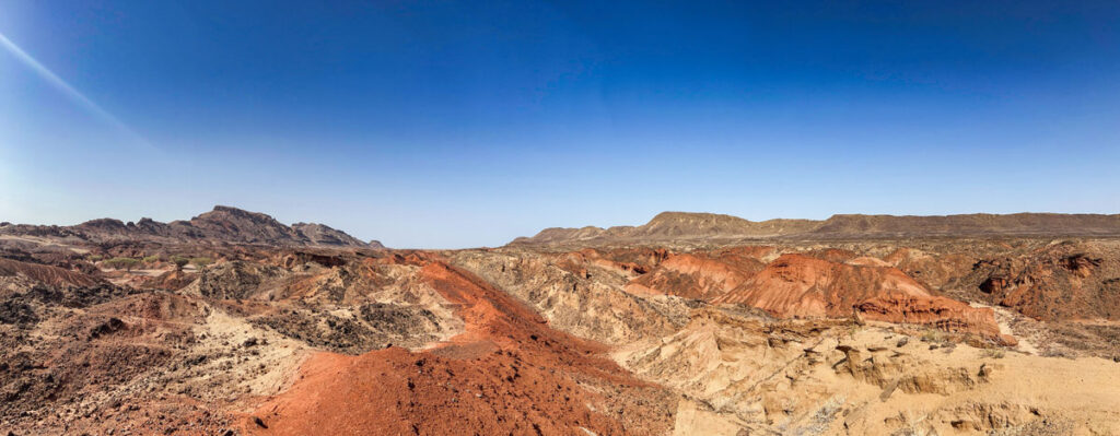
The Lothagam site in the Turkana Rift Zone contains tilted sediments from the late Miocene (about 7 million years ago), just before the necking phase of rifting commenced. Credit: Christian Rowan
Breaking Up Is Hard to Do
Just like mid-ocean ridges on the seafloor, sections of Earth’s crust on land also stretch apart as tectonic plates separate. This process, called rifting, takes place in three stages. First, the crust stretches, creating tension. Then it rapidly thins like pulled taffy—this is the necking stage. Finally, magma wells up from the lithospheric mantle, which creates new seafloor and breaks the continental plate apart.
“This is one of the unique places on Earth where you can see a continental rift.”
Not every rift makes it that far. Some remain stuck in the stretching phase with crust more than 20 kilometers thick. But northern sections of the East African Rift System (EARS), specifically the Afar Rift and the Red Sea, are already undergoing the final stage, oceanization.
“This is one of the unique places on Earth where you can see a continental rift,” said Anne Bécel, a geophysicist at Lamont-Doherty Earth Observatory of Columbia University in Palisades, N.Y., and coauthor of new research published in Nature Communications in April. “The East African Rift System has been studied for a very long time by geologists to really learn about our planet and how continents break apart, and then transpose that to mid-ocean ridges where oceanic plates spread apart.”
The team suspected that the Turkana Rift Zone, located at a critical triple junction in northern Kenya, was behaving differently from other areas of the rift system. It is home to an unusually large and continuous hominin fossil record dating back about 4 million years. Past research has also shown that the bottom of the crust, called the Moho, is unusually shallow in the Turkana Basin, just 20 kilometers deep compared with the average depth of 39 kilometers farther away from the rift.
During several field expeditions to Lake Turkana in partnership with local industries, the team mapped the top of the continental crust using borehole measurements and seismic reflection—sending seismic waves into the ground and measuring how the waves bounce back, like sonar. They combined those measurements with past research into Moho depths to calculate the crustal thickness near Lake Turkana.
That map showed that far away from the rift, the crust is more than 35 kilometers thick, but in the Turkana Rift Zone it is a mere 13 kilometers thick, below the threshold for necking.
“If you look at the modern day topography, the whole East African Rift is in this really low, broad land between two big plateaus, one to the north in Ethiopia and one towards the south,” said lead researcher Christian Rowan, a geologist and doctoral candidate at Columbia University. “It’s this very strange topographic feature, and part of that low-lying topography is actually how thin the crust is there.”
“The oldest rocks that record the initiation of the East Africa Rift System are also in the Turkana Rift,” said coauthor Folarin Kolawole, a Columbia University geologist. Geochemical analysis of those rocks suggests that necking in the Turkana Rift Zone began about 4 million years ago.
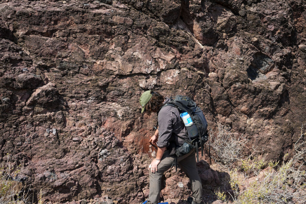
Christian Rowan measures a fault in the Turkana Rift. Credit: Christian Rowan
About to Break?
“Any time you have a place on the planet that is rare in the modern but seen in the past, it is compelling,” said Erik Klemetti Gonzalez, a volcanologist at Denison University in Granville, Ohio, who was not involved with this research. “The data does show that the Turkana Rift is the home of anomalously thin continental crust, so if you are looking for a location that meets criteria for necking, it seems to be the case.”
The team suspects that Turkana might have been primed to split apart more easily because another rifting event took place there a mere 17 million years before the present rift began. The Turkana Basin inherited a weaker section of crust that didn’t have time to fully heal in the (geologically) short time between rifting events. There was also an extended period of magmatic activity throughout much of the past 45 million years.
“Magmatism is well known to be a significant weakening factor in rifting,” Rowan said. “I think the two compounding effects of this inheritance and then magnetism is why the Turkana rift is so much more mature than other segments.”
“I would hope that more collaboration with African geoscientists could create the ability to collect data from places that have been more inaccessible over the past half century.”
“There are many ‘failed rifts’ in the geologic record, so the question of whether the EARS is actually leading to a continental break up, albeit a small one, is still very much up in the air,” Klemetti Gonzalez said. These new results tip the scales toward breakup, but he noted that more of the rift system still needs to be mapped to really understand the fate of this region.
“I would hope that more collaboration with African geoscientists could create the ability to collect data from places that have been more inaccessible over the past half century,” he added.
Rowan and his team are working toward that end by continuing to map crustal thicknesses in other nearby rift zones.
“This was the only known rift that was undergoing necking along the entire East African Rift System, or in the world,” said Kolawole. “But based on ongoing work, there is evidence that there are other segments that are at the onset of necking in the East African Rift System.”
Citation: Cartier, K. M. S. (2026), Eastern Africa is splitting apart, but not where we expected, Eos, 107, https://doi.org/10.1029/2026EO260148. Published on 12 May 2026.