Editors’ Highlights are summaries of recent papers by AGU’s journal editors.
Source: AGU Advances
The albedo change of marine clouds is achieved by targeted additions of aerosols, and in particular, sea salt. To assess the viability of Marine Cloud Brightening (MCB) requires a fundamental understanding of the impact of aerosols on cloud evolution and properties, and on the cloud environment.
Doherty et al. [2026] propose a framework for studying MCB across scales. This includes small-
The albedo change of marine clouds is achieved by targeted additions of aerosols, and in particular, sea salt. To assess the viability of Marine Cloud Brightening (MCB) requires a fundamental understanding of the impact of aerosols on cloud evolution and properties, and on the cloud environment.
Doherty et al. [2026] propose a framework for studying MCB across scales. This includes small- to large-scale studies aimed at systematically characterizing the life-cycle of aerosols and the diurnal cycle of cloud processes, how these change with the magnitude, duration and type of aerosol applied, and monitoring potential harmful direct or indirect consequences of aerosol injection, such as regional changes in temperature or precipitation.
Possible configuration for a Stage III study for measuring local scale cloud responses to a single plume of generated sea salt aerosol sized for marine cloud brightening. Credit: Doherty et al. [2026], Figure 4
Citation: Doherty, S. J., Diamond, M. S., Wood, R., & Hirasawa, H. (2026). Defining scales of field studies and experiments to assess marine cloud brightening. AGU Advances,7, e2025AV001939. https://doi.org/10.1029/2025AV001939
Editors’ Highlights are summaries of recent papers by AGU’s journal editors.
Source: Journal of Geophysical Research: Atmospheres
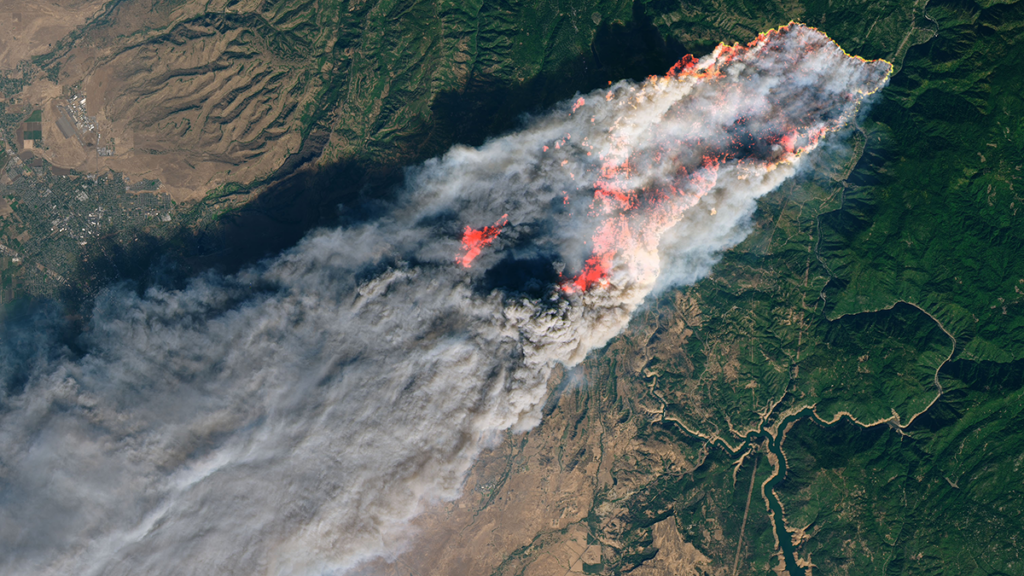
The 2018 Camp Fire was the deadliest and most destructive wildfire in California history. The Camp Fire spread extremely rapidly, driven by strong winds and dry fuels, but also by organized long-range spotting, i.e. lofting and downwind fallout of burning embers to ignite new fires.
Using operational Doppler radar and satellite observations, Lareau [2026] pr
Source: Journal of Geophysical Research: Atmospheres
The 2018 Camp Fire was the deadliest and most destructive wildfire in California history. The Camp Fire spread extremely rapidly, driven by strong winds and dry fuels, but also by organized long-range spotting, i.e. lofting and downwind fallout of burning embers to ignite new fires.
Using operational Doppler radar and satellite observations, Lareau [2026] provides the first high resolution depiction of spotting behavior during an extreme wildfire. Observations show that spot fire events for the Camp Fire occurred 5-10 kilometers ahead of the fire front, quickly merging into new fire lines. Spot fires are not random but aligned within coherent fallout zones that are shaped by plume dynamics and background winds. These results show that operational weather radar can identify lofting and fallout regions in real time, providing a new way to anticipate spotting-driven fire spread and improve early warnings for fast-moving wildfires.
(a) Along wind cross section of Camp Fire plume reflectivity observed by radar measurements, showing distinct updrafts (white arrows) and ashfall regions (blue dashed arrow). Spot fires within 10 minutes of these radar measurements are shown as filled cyan triangles. (b) Map of column maximum radar reflectivity and fire perimeter. In both panels the black dashed line indicates the eastern edge of the town of Paradise, California. Credit: Lareau [2026], Figure 6ab
Citation: Lareau, N. P. (2026). Plume-coupled long-range spotting drove the explosive spread of the 2018 Camp Fire. Journal of Geophysical Research: Atmospheres, 131, e2025JD045798. https://doi.org/10.1029/2025JD045798
Editors’ Vox is a blog from AGU’s Publications Department.
Ensuring the sustainability of water resources and ecosystems in a changing world requires a thorough understanding of how water moves through Earth’s Critical Zone, a dynamic interface where air, water, soil, plants, and rocks interact. Researchers can track and model this movement of water using naturally occurring markers or “tracers.”
A recent article in Reviews of Geophysics explores the latest advancements in tracer-aided mi
Ensuring the sustainability of water resources and ecosystems in a changing world requires a thorough understanding of how water moves through Earth’s Critical Zone, a dynamic interface where air, water, soil, plants, and rocks interact. Researchers can track and model this movement of water using naturally occurring markers or “tracers.”
A recent article in Reviews of Geophysics explores the latest advancements in tracer-aided mixing models and how they can help us to better understand the Critical Zone. Here, we asked the authors to give an overview of the Critical Zone, how tracer-aided mixing modeling works, and future directions for research.
What is the Critical Zone (CZ)?
The Critical Zone is Earth’s “living skin”—the dynamic layer where the atmosphere, hydrosphere, biosphere, and lithosphere interact. It stretches from the top of the vegetation canopy and, in cold regions, from the surface of snowpacks and glaciers, down through soils and into the deeper aquifers. It encompasses lakes, streams, and wetlands at the surface, and extends beyond the soil layer to underlying groundwater aquifers. It is where rainfall, snowmelt and glacier melt become soil moisture, where plants take up water and return it to the atmosphere, where aquifers get recharged, and where streamflow is generated. In short, the Critical Zone is where most processes that sustain terrestrial life and freshwater resources unfold.
Why is it important to understand how water moves through the Critical Zone?
Virtually every freshwater resource we rely on (e.g., drinking water, irrigation) passes through the Critical Zone.
Virtually every freshwater resource we rely on (e.g., drinking water, irrigation) passes through the Critical Zone at some point. Global warming, land-use changes, and intensifying water demand emerging from rapid urbanization and changes in agriculture are reshaping how water is stored and released within the Critical Zone, often in ways we cannot yet predict. Understanding how much water is stored within the Critical Zone, how this water is both recharged from rainfall and snowmelt and eventually discharged into streams, and the timescale of these dynamic processes is essential for protecting ecosystems, safeguarding water supplies, and adapting to a changing climate.
How would you explain a tracer-aided mixing model to a non-specialist?
Imagine mixing a glass of orange juice with a glass of apple juice, and trying afterwards to work out how much of each went into the glass. If the juices had distinctive “fingerprints” (imagine its color, sugar content, or a specific chemical) and these fingerprints primarily changed because of the mixing of these two juices, you can then measure the fingerprint in the final mixture and back-calculate the proportion of its distinct sources.
Tracer-aided mixing models work in a similar way but can track the entire water cycle. Different water sources (e.g., rainfall, snowmelt, glacier melt, soil water, groundwater) can have distinct “fingerprints” in a naturally occurring tracer, such as stable isotopes of water or specific dissolved elements. By measuring these fingerprints in the streamwater or groundwater and in its potential sources for example, hydrologists can estimate how much each source contributed to the streamwater or groundwater.
Conceptual model of the different components of the Critical Zone. “Gw” stands for groundwater. Credit: Popp et al. [2025], Figure 2
What are some of the most significant and exciting recent advances in tracer-aided mixing models?
Classical mixing models relied on demanding assumptions: that all water sources can be identified and sampled, and that their signatures were distinct and constant in time. Much of the recent progress has been about relaxing these assumptions.
Bayesian approaches now estimate full probability distributions and provide a more realistic picture of uncertainty. Methods like Convex Hull End-Member Mixing Analysis (CHEMMA) use machine learning to infer the distinct sources directly from data, while ensemble hydrograph separation exploits tracer fluctuations over time, thereby making un-mixing feasible even when multiple sources have overlapping signatures. Perhaps the most conceptually novel advance is end-member splitting, which flips the question from “where does streamflow come from?” to “where does precipitation go?”
Alongside these modeling advances, there have been immense advances in how tracers are measured. Portable laser and mass spectrometers now enable high-frequency, in-situ tracer measurements which allows us to capture critical hydrological events such as storms and snowmelt in near-real time.
What are stable water isotope tracers and what are their advantages?
Stable water isotopes are naturally occurring non-radioactive atoms of hydrogen and oxygen that make up a water molecule but have slightly different molecular masses. The two stable isotopes widely used in hydrology are 2H (deuterium) and 18O (oxygen-18). Because these isotopes are part of the water molecule itself, they directly travel with the water molecule. Their key advantages are: (1) they are conservative, meaning they do not react chemically as water moves through soils and aquifers, and (2) they carry distinct signatures resulting from climatic variables such as air temperature.
These properties make stable water isotopes the most versatile and widely used tracer in Critical Zone hydrology.
Consequently, in the European Alps, winter precipitation has a different isotopic signature than summer precipitation because winters are cooler than summers. Other hydrological processes such as evaporation and sublimation leave a recognizable fingerprint on the remaining water, thereby allowing us to estimate how much evaporation or sublimation occurred. Stable water isotopes can be measured in essentially every water compartment, from atmospheric vapor and precipitation to snowpack, plant xylem, soil water, streams, and groundwater. Together, these properties make stable water isotopes the most versatile and widely used tracer in Critical Zone hydrology.
What are the current limitations of tracer-aided mixing models?
Despite their power, mixing models still face many constraints. End-member signatures vary in space and time, are sometimes too similar to distinguish, and some sources may be overlooked entirely. Non-conservative tracers such as nitrate or sulfate can react with their environment along their journey, thereby biasing results if these reactions are not explicitly accounted for.
Sampling is another major bottleneck. Capturing the spatial heterogeneity of soils, snowpacks, and groundwater requires a lot of measurements that are often logistically or financially prohibitive, especially in remote regions. Many of the newer, more powerful tracers such as noble gases or stable isotopes of trace elements, can only be analyzed by a handful of specialized laboratories. As a result, global coverage remains highly uneven, with key regions such as the Arctic and the global South still under-sampled.
What are some of the major unsolved questions and where is more research needed?
There are several fronts where more research is needed. Source signatures are not static, and methods that explicitly capture their variability in time are still underdeveloped. Embedding tracers within global Earth System Models would, in theory, enable more accurate assessment of hydrological partitioning e.g., how rainfall, snowmelt, and glacier melt are split between sublimation, evapotranspiration, groundwater, and streamflow. These will directly inform more robust climate projections, but this remains technically demanding.
Expanding data coverage in under-sampled regions is critical, and citizen science and low-cost sensors may help. Machine learning is a promising approach for uncovering non-linear relationships and gap-filling sparse datasets, but requires training data that often do not yet exist. Greater interdisciplinary integration, e.g., combining tracers with remote sensing, ecological indicators, and biogeochemical data, could yield a more holistic view of the Critical Zone. Finally, the field would benefit from shared protocols and open data practices to enhance progress.
Editor’s Note: It is the policy of AGU Publications to invite the authors of articles published in Reviews of Geophysics to write a summary for Eos Editors’ Vox.
Citation: Popp, A. L., and H. Beria (2026), Tracing water’s hidden journey through the Earth’s living skin, Eos, 107, https://doi.org/10.1029/2026EO265019. Published on 13 May 2026.
This article does not represent the opinion of AGU, Eos, or any of its affiliates. It is solely the opinion of the author(s).
Editors’ Highlights are summaries of recent papers by AGU’s journal editors.
Source: Journal of Geophysical Research: Atmospheres
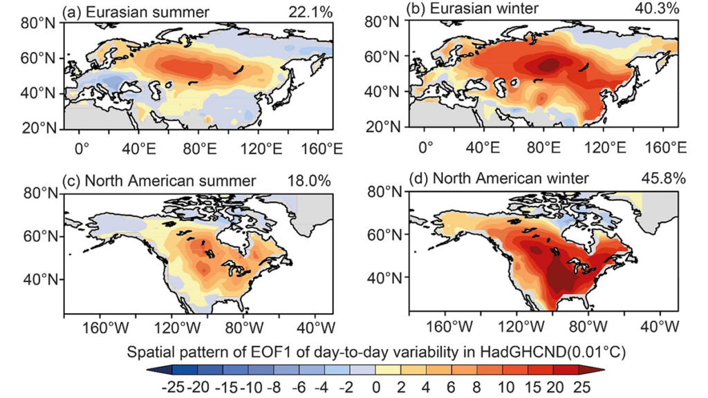
Abrupt temperature swings between consecutive days, referred to as day-to-day temperature variability, have far-reaching impacts on human health, ecosystems, and economic activity. However, how these fluctuations vary from year to year, and what drives them, has remained unclear.
Using observations, reanalysis, and CMIP6 simulations from 1961 to 2014, Liu an
Source: Journal of Geophysical Research: Atmospheres
Abrupt temperature swings between consecutive days, referred to as day-to-day temperature variability, have far-reaching impacts on human health, ecosystems, and economic activity. However, how these fluctuations vary from year to year, and what drives them, has remained unclear.
Using observations, reanalysis, and CMIP6 simulations from 1961 to 2014, Liu and Fu [2026] identify a coherent large-scale pattern of variability across Eurasia and North America. This variability is primarily driven by the north–south movement of warm and cold air masses.
The dominant drivers also vary by season: large-scale meteorological patterns prevail in winter, whereas local land–atmosphere feedbacks become more influential in summer. Together, these processes reshape temperature gradients and modulate storm activity and broader weather systems.
Overall, the findings provide new insights into the mechanisms of temperature variability and offer a scientific basis for improving seasonal climate risk prediction and adaptation strategies.
Citation: Liu, Q., & Fu, C. (2026). Interannual variations in the day-to-day temperature variability in the northern hemisphere and possible causalities. Journal of Geophysical Research: Atmospheres, 131, e2025JD045754. https://doi.org/10.1029/2025JD045754
Research & Developments is a blog for brief updates that provide context for the flurry of news regarding law and policy changes that impact science and scientists today.
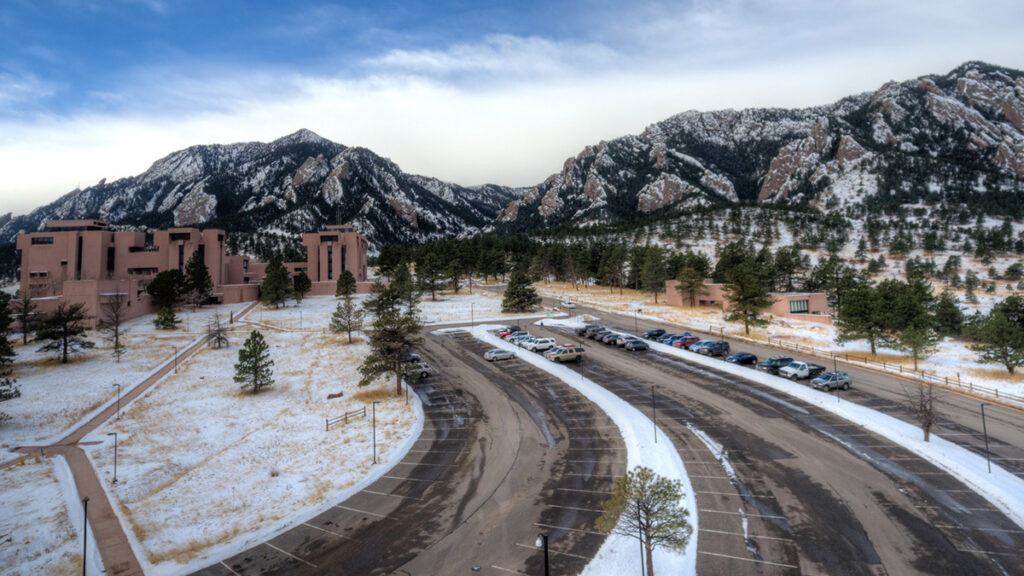
A Colorado judge has granted a preliminary injunction to the University Corporation for Atmospheric Research (UCAR). The move temporarily blocks the federal government from moving forward with one part of its effort to dismantle UCAR’s National Center for Atmospheric Research (NCAR) by transferring stewardship of a
Research & Developments is a blog for brief updates that provide context for the flurry of news regarding law and policy changes that impact science and scientists today.
A Colorado judge has granted a preliminary injunction to the University Corporation for Atmospheric Research (UCAR). The move temporarily blocks the federal government from moving forward with one part of its effort to dismantle UCAR’s National Center for Atmospheric Research (NCAR) by transferring stewardship of a state-of-the-art supercomputing facility.
Together, UCAR—a nonprofit consortium of universities and colleges—and the National Science Foundation (NSF) operate and maintain the NCAR-Wyoming Supercomputing Center (NWSC) in Cheyenne, Wyo. The facility provides scientists with enormous computational power necessary to run sophisticated analyses of weather, climate, and other Earth systems.
In February, as another step in a chain of actions taken to dismantle NCAR, the NSF informed UCAR and NCAR that it would transfer management and operations of NWSC to a third-party operator.
In turn, UCAR filed a lawsuitalleging that the action violated federal law under the Administrative Procedure Act (APA). To halt NSF’s action under the act, the agency’s attempt to remove UCAR’s stewardship of the facility must be shown to be “arbitrary, capricious, an abuse of discretion, or otherwise not in accordance with law.”
Judge Richard Brooke Jackson of the U.S. District Court for the District of Colorado wrote in a 1 June court order that the action was both arbitrary and capricious “for at least two reasons.” First, NSF didn’t offer an explanation for its decision, and second, it didn’t follow an outlined process to consider public feedback.
The decision means that UCAR will temporarily retain its stewardship of NWSC.
“NSF’s failure to provide any explanation for its decision—let alone a reasonable one—thwarts meaningful judicial review and renders the challenged action arbitrary and capricious,” Jackson wrote.
He went on to note that efforts to transfer stewardship of UCAR assets, including the supercomputing center, to other institutions, pose the risk of “irreparable harm” to UCAR. One of the chief harms would be brain drain, the judge noted multiple times, writing that “UCAR cannot easily replace employees with the level of education, specialized training, and institutional knowledge necessary to operate and maintain the NWSC’s ‘highly integrated, high-performance supercomputing system.'”
In addition to brain drain, Jackson cited financial injuries to UCAR that would be “difficult, if not impossible” to quantify, as well as an overall threat to the consortium’s mission.
“Any degradation in forecasting, modeling, or related scientific capabilities carries real-world consequences, including potential harm to property and human life. Given those stakes, the public interest strongly favors maintaining the status quo unless and until NSF demonstrates that its transfer decision complies with the APA,” he concluded.
In a statement posted to the UCAR website, the consortium’s interim president, Eric Barron, said UCAR was pleased that Judge Jackson recognized how harmful the proposed transfer would be for the the nation’s scientific enterprise.
“UCAR’s top priority is to advance Earth system science in service to society,” he wrote. “Today’s decision ensures that the NWSC will be able to continue its vital work on behalf of the United States and its stakeholders without interruption.”
These updates are made possible through information from the scientific community. Do you have a story about how changes in law or policy are affecting scientists or research? Send us a tip at eos@agu.org.
Seeking Solutions to PFAS Pollution
Chemical Companies Are Churning Out New PFAS. Where in the World Are They Ending Up?
The Persistence of PFAS
A Peculiar Polymer Paired with Sunlight Could Remove PFAS
Tracing the Path of PFAS Across Antarctica
Pollution Is Rampant. We Might As Well Make Use of It.
Per- and polyfluoroalkyl substances (or PFAS) have been widely used in thousands of common nonstick, waterproof, or stain-resistant products since the 1950s. These “forever c
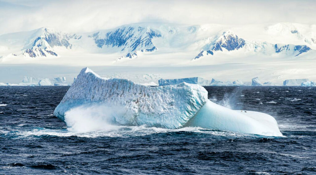
Per- and polyfluoroalkyl substances (or PFAS) have been widely used in thousands of common nonstick, waterproof, or stain-resistant products since the 1950s. These “forever chemicals” do not break down easily: PFAS make their way into the air, soil, and water, as well as into human and animal bloodstreams and to some of Earth’s most pristine environments. They have been detected even in Antarctica, despite its reputation as a relatively untouched landscape far from the types of products—fast-food wrappers, firefighting foam, nonstick cookware—that contain PFAS.
Research into how PFAS arrive in Antarctica is limited, and most tends to focus on the continent’s coasts, rather than its interior. A new study published in Science Advances aimed to fill some of these gaps by examining PFAS accumulation across a 1,200-kilometer stretch of Antarctica, from the snow pits of Zhongshan Station in East Antarctica to the 4,093-meter peak of Dome A. By examining layers of snow collected from the coast to the interior, researchers sought to better track and understand how PFAS levels vary by location and how these forever chemicals have been able to travel long distances through the upper atmosphere to be deposited in remote regions.
“For substances to get there, they have to be able to transport long distances,” said Ian Cousins, a chemist at Stockholm University and one of the study’s authors. “We know PFAS are very persistent, so that helps. By looking at the patterns of the PFAS contamination in the samples, it gives us clues as to how they’re transported.”
PFAS Arrive by Air and by Sea
Along the 1,200-kilometer route, researchers from the Chinese Academy of Sciences collected 39 snow samples at 30-kilometer intervals, scraping the first few centimeters of snow from the surface to analyze for traces of PFAS.
Zhongshan Station sits near Prydz Bay, and there, researchers collected snow from a 1-meter-deep pit, with samples taken every 5 centimeters. At Dome A, the summit of the East Antarctic Ice Sheet, samples were collected at 10-centimeter intervals from another snow pit; this one was 3 meters deep, providing information about the past several decades of PFAS use.
“It’s quite interesting that we see the historical production record of PFAS in this pit on the top of this mountain in Antarctica,” said Cousins.
PFAS pollution arrives in Antarctica in two ways: via upper atmospheric transport and sea spray. Some PFAS are formed in the atmosphere when volatile precursor chemicals like fluorotelomer alcohols used in textile and paper products break down through reactions with sunlight and oxidants into more stable compounds. The resulting PFAS are later deposited into the snow and ice through precipitation.
Storm winds near the coast create sea spray. “When you have waves, it makes bubbles in the ocean. When the bubbles burst, these sea spray aerosols can be super enriched with PFAS. This has been shown to be a very important transport route,” Cousins said.
To distinguish between sources, researchers measured sodium in the snow to trace the ocean’s salty influence. Sodium levels decreased farther inland, reflecting the fading influence of sea spray toward the interior of the continent. But surprisingly, PFAS concentrations actually increased moving from the coast into the interior.
“That was kind of a bit counterintuitive to me,” explained Cousins, who said he expected PFAS levels to be highest near the coast. “You see the opposite, actually.”
The inland increase is likely explained by higher snowfall totals in the coastal regions, which lead to PFAS concentrations becoming diluted. Inland, where snowfall is lower, even small amounts of PFAS can result in relatively higher concentrations within snow samples.
Additional factors shape PFAS distribution. PFAS levels are higher at the onset of precipitation events when they are rapidly removed from the air. Temperature inversions, too, can trap chemicals. In coastal areas, PFAS are more influenced by sea spray in the winter, whereas stronger sunlight drives the degradation of atmospheric precursors into PFAS in the summer months.
PFAS Presence at Both Poles
This new study also offers implications for the way that PFAS circulate globally. Though industrial activity in the Northern Hemisphere contributes most heavily to PFAS emissions, large-scale atmospheric circulation allows these compounds to reach polar regions. Rapid transport in the upper troposphere may act as an efficient pathway to shuttle PFAS across both hemispheres before they are deposited in the cold, remote regions at both ends of Earth.
“This completes the global picture with agreeing measurements at both poles, solidifying our understanding of the global distribution and drivers of PFAS contamination.”
Even though PFAS levels are higher in the Arctic, both polar regions show similar trends in PFAS concentrations since the 1990s. “It really matches decades of the same records that have been reported from the Arctic,” said Cora Young, an atmospheric chemist at York University, who was not involved in the new study.
“This completes the global picture with agreeing measurements at both poles, solidifying our understanding of the global distribution and drivers of PFAS contamination. The role of CFC [chlorofluorocarbon] replacements, changes in regulation, all of these things are important in the Northern Hemisphere and also the Southern Hemisphere,” said Young.
Source: Geophysical Research Letters
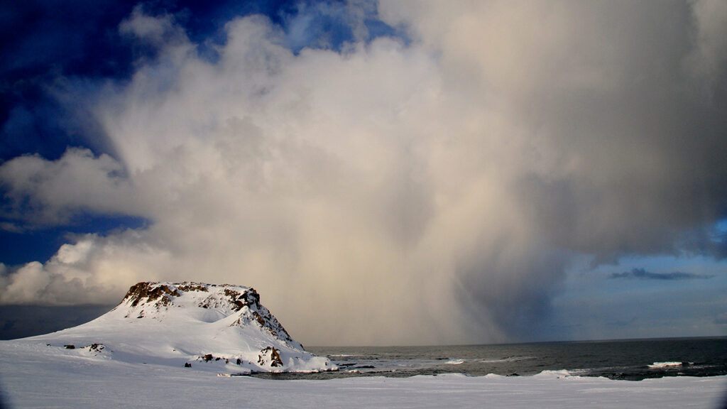
Atmospheric rivers act like “rivers in the sky,” shuttling intense bands of warm, heavy moisture from lower to higher latitudes. When an atmospheric river encounters cold air or mountainous terrain, the moisture it carries condenses and falls as heavy rain or snow. In Antarctica, the arrival of an atmospheric river can help build surface ice mass. Much of Antarctica is very dry; an atmospheric river can bring the moisture needed to potentially offset some
Atmospheric rivers act like “rivers in the sky,” shuttling intense bands of warm, heavy moisture from lower to higher latitudes. When an atmospheric river encounters cold air or mountainous terrain, the moisture it carries condenses and falls as heavy rain or snow. In Antarctica, the arrival of an atmospheric river can help build surface ice mass. Much of Antarctica is very dry; an atmospheric river can bring the moisture needed to potentially offset some ice loss.
Antarctica’s varied topography and dry conditions have made detecting atmospheric rivers over the continent challenging. Previous efforts to do so have suggested that atmospheric rivers contribute up to 30% of Antarctica’s total annual precipitation, but these methods may not be capturing the full picture of atmospheric river activity.
Takahashi et al. developed a new 3D atmospheric river detection algorithm to better capture how atmospheric rivers affect Antarctica’s complex terrain. Previous methods have mostly been 2D, meaning they do not accurately account for the vertical variations within an atmospheric river.
To evaluate the algorithm, the researchers applied it to two datasets: (1) daily snowfall totals measured during the 44th Japanese Antarctic Research Expedition (JARE44) at Dome Fuji from February 2003 to January 2004 and (2) the ERA5 (European Centre for Medium-Range Weather Forecasts atmospheric reanalysis) dataset of daily weather patterns and conditions in Antarctica from 1979 to 2023.
The results of the study’s new algorithm showed 16 significant snowfall events during the JARE44 expedition, all of which were not detected by the older 2D method. The new 3D method identified 17 days of atmospheric river activity, which corresponded with 10 heavy snowfall events and accounted for approximately 40% of the total precipitation. Between 1979 and 2023, atmospheric rivers occurred about 10% of the time yet contributed 30%–60% of total precipitation in the Antarctic interior.
The 3D method in the new study suggests that atmospheric river events contribute a greater proportion of total snowfall than previously thought—between 30% and 90%, depending on the Antarctic region. The researchers also suggest that long-term changes in Antarctic snowfall are closely linked with the changes in atmospheric river activity. This connection is especially apparent in East Antarctica, where the link between snowfall increases and atmospheric rivers had not yet been clearly identified in previous studies. (Geophysical Research Letters, https://doi.org/10.1029/2025GL120986, 2026)
“I’ve just always felt like art and science are flip sides of the same coin.”
Scientists use tools ranging from models to microscopes to make sense of the world around them. Some might say artists do the same thing using tools such as paintbrushes and musical instruments.
“I’ve just always felt like art and science are flip sides of the same coin, with maybe different outcomes or different processes, but they’re both just getting at the truth of the world,” said Sara Bouchard, a sound art
“I’ve just always felt like art and science are flip sides of the same coin.”
Scientists use tools ranging from models to microscopes to make sense of the world around them. Some might say artists do the same thing using tools such as paintbrushes and musical instruments.
“I’ve just always felt like art and science are flip sides of the same coin, with maybe different outcomes or different processes, but they’re both just getting at the truth of the world,” said Sara Bouchard, a sound artist and composer and adjunct faculty member in the Department of Kinetic Imaging at Virginia Commonwealth University’s (VCU) School of Art.
A recent National Science Foundation–funded collaboration between scientists and artists brought this principle to life.
In fluxART, artists partnered with scientists from FLUXNET, an international network of researchers using eddy covariance techniques to measure how gases move between ecosystems and the atmosphere.
Researchers and artists collaborated on art projects based on data collected at FLUXNET towers. A view from the top of one such tower near Sisters, Ore., is seen here. Credit: Alexander Irving
The scientist-artist pairs worked together in yearlong residencies and produced art pieces—ranging from music compositions and video installations to ceramic works and paintings—that they presented at the Patricia Valian Reser Center for the Creative Arts in Corvalis, Ore., in early 2026.
“Part of the framing of the residency was around flux as this metaphor for connection and belonging and relationships.”
“The metaphor that people use to describe what this science network measures, or does, is that it’s monitoring the breath of the biosphere,” said Maoya Bassiouni, an environmental scientist at the University of California, Berkeley, who directed and developed the residency. “Those fluxes are sort of this giving and receiving between the land and the atmosphere, and it’s exactly what the scientists are doing in the community. So, part of the framing of the residency was around flux as this metaphor for connection and belonging and relationships.”
Bassiouni, who also created artworks in the residency, presented a lecture about the series alongside two other fluxART artists in late May at the National Center for Atmospheric Research’s (NCAR) Mesa Lab in Boulder, Colo.
An installation at NCAR’s Mesa Lab Library featuring all four fluxART projects also opened on 27 May and will be on display through the end of 2026.
En Masse
Bouchard, the sound artist, was paired with Chris Gough, a biogeochemist who serves as the executive director of the Rice Rivers Center at VCU.
Gough studies how factors such as climate and disturbances affect ecosystems, particularly forests and wetlands. Bouchard learned more about Gough’s work by spending a year in his lab.
Virginia Commonwealth University’s Rice Rivers Center Marsh, an AmeriFlux site whose data were used in this project, is located along the James River, seen here. Credit: Megan May Photography
The result was a composition for choir and percussion called En Masse, which explores the connections between communities and ecosystems in a time of climate crisis. The piece’s five movements represent the movement of carbon through the environment: “Air,” “Wood,” “Soil,” “Fire,” and “Breath.”
In addition to vocals and instruments, the composition features birdsong, recordings from a compost pile, sonified data from Gough’s lab, and spoken words gathered from real people sharing their climate anxieties. An excerpt from the “Fire” movement reads,
Future! / Heavy weight on my ribcage / dusty, fragmented Fire! / Clenched jaw, copper taste in my mouth / stark, shifted Fire! / I worry about my kids / desperate, unbreathable Fire! / and their future / squeezed, extreme Future! Fire! Fire! Fire!
Both Bouchard and Gough said they were moved by the piece as it was performed in Corvalis and by seeing the mix of artists and scientists who attended, many traveling from other states.
“I was struck by how engaged both the scientific and artistic communities were,” Gough said. “We walked out, and it was a full room of people. It was energizing, and I think it felt meaningful in a way that stepping up on a conference stage to deliver the traditional convention talk [isn’t].”
September: Orange
In another pairing, video artist Julia Oldham partnered with Christopher Still, a plant ecophysiologist at Oregon State University.
The partnership started with Oldham visiting a 175-foot-tall (53-meter-tall) FLUXNET tower near Sisters, Ore., that Still and his team monitor.
Video artist Julia Oldham visited a FLUXNET tower near Sisters, Ore., with scientist Christopher Still in preparation for creating an art piece based on data gathered at the tower. Credit: Alex Irving
At the top of the tower, a PhenoCam takes photos of the surrounding Deschutes National Forest every half hour. Still uses data from these images to examine how the greenness of the canopy changes over time because such changes can provide information about fluxes in carbon, water, and energy.
“I learned more about what Chris uses the PhenoCam for and got superexcited about the fact that Chris is using color data to understand forests,” Oldham said. “I thought that that was a really beautiful point of overlap for us as a scientist and an artist, to think about color and forests and what we can learn from color as a scientific tool.”
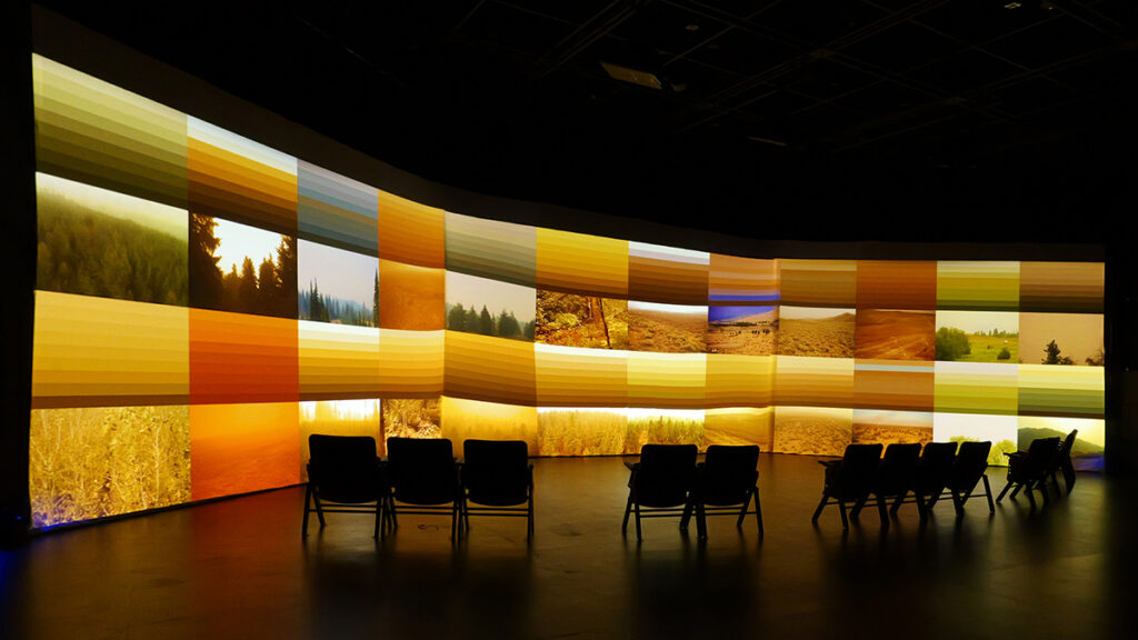
The pair created two pieces. 18//Flux shows how the colors and light from one PhenoCam site changed from 4 a.m. to 9 p.m. throughout the year for 13 years. Each frame is divided into 13 strips, with each strip representing 1 hour of the monitoring period.
The two had conversations throughout the duration of the project about the growing role of wildfires in the area. In fact, one of the FLUXNET towers they were using in the project burned down.
Their conversations led to September: Orange, a three-channel video showing footage from 24 different PhenoCams in the northwestern United States and Canada. When all of the landscapes are the same shade, the video briefly pauses. In September, when wildfires sweep through Cascadia, orange becomes the dominant color. The piece is accompanied by field recordings from Oregon forests and sonified canopy greenness data.
“I think the installation was a wild success, and I had a lot of people tell me how much they enjoyed it and appreciated it,” Still said. “Most people don’t respond to a 2D graph of data…whereas I think almost everyone responds to images, and photographs are really meaningful to people. So I think that is a really brilliant way to draw people into the science.”
Citation: Gardner, E. (2026), Artists and scientists partner to bring atmospheric data to life, Eos, 107, https://doi.org/10.1029/2026EO260178. Published on 3 June 2026.