Ironbridge - River Severn
28 May 2026 at 20:08


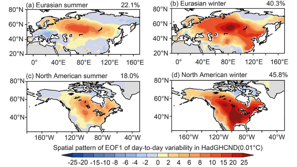
Abrupt temperature swings between consecutive days, referred to as day-to-day temperature variability, have far-reaching impacts on human health, ecosystems, and economic activity. However, how these fluctuations vary from year to year, and what drives them, has remained unclear.
Using observations, reanalysis, and CMIP6 simulations from 1961 to 2014, Liu and Fu [2026] identify a coherent large-scale pattern of variability across Eurasia and North America. This variability is primarily driven by the north–south movement of warm and cold air masses.
The dominant drivers also vary by season: large-scale meteorological patterns prevail in winter, whereas local land–atmosphere feedbacks become more influential in summer. Together, these processes reshape temperature gradients and modulate storm activity and broader weather systems.
Overall, the findings provide new insights into the mechanisms of temperature variability and offer a scientific basis for improving seasonal climate risk prediction and adaptation strategies.
Citation: Liu, Q., & Fu, C. (2026). Interannual variations in the day-to-day temperature variability in the northern hemisphere and possible causalities. Journal of Geophysical Research: Atmospheres, 131, e2025JD045754. https://doi.org/10.1029/2025JD045754
—Yun Qian, Editor, JGR: Atmospheres
The key word here is could. Experts including Ken Graham, the director of NOAA’s National Weather Service, all emphasize that no two El Niños are alike.
“Each one is unique with its own imprint on our weather,” Graham said in a NOAA press release. However, scientists have learned a few things from watching the ways that this warm phase of a natural climate cycle over the tropical Pacific has affected our weather patterns in the past.
“Advanced monitoring and an improved understanding of El Niño patterns allow the NWS to better predict and better prepare the public and our core partners for what is to come,” Graham said.
This morning, NOAA released an El Niño Advisory, announcing that the climate phenomenon (the warm phase of the El Niño–Southern Oscillation) has officially arrived in the tropical Pacific. The agency forecasts a 63% chance of a “very strong” El Niño from November 2026 to January 2027 that “would rank among the largest El Niño events in the historical record.”
NOAA defines a “very strong” El Niño as when the Pacific’s surface waters are more than 2°C warmer than average. The agency doesn’t use the phrase “Super El Niño,” but there have only been three such “super” or “very strong” El Niño events since 1980. The last one was in 2015.
What does this mean for climate, for humans, and marine species? Here’s a roundup of some potential forecasted effects—some good, some bad—of the weather pattern that’s been making headlines over the past few months.
In a typical year, a warm pool of water in the equatorial Pacific would be transported westward—away from the western coast of the Americas—by trade winds. But during an El Niño event, those trade winds weaken, and the warm pool of water extends east, explained Ariel Cohen, the meteorologist in charge of the National Weather Service’s Los Angeles and Oxnard Office in a press briefing at the Aquarium of the Pacific in Long Beach, Calif.
This warm water “causes jet energy in the atmosphere to bring disturbed weather southward across the southern United States, which can bring wetter than normal conditions to our area with drier conditions farther to the north,” Cohen said.
The southward shift of the storm track could also lead to drier conditions over the northern Rockies and as far east as the Ohio and Tennessee Valleys.
In the past, strong El Niños have led to decreased amounts of plankton in the Pacific, particularly the open ocean, forcing species that rely on plankton (and the species that rely on the species that rely on plankton, and so forth) to widen their net when searching for food.
“[Plankton] is important because that’s the base of the food web,” explained Andrew Leising, a research oceanographer at NOAA, at the Aquarium of the Pacific. “Marine mammals and other migratory species end up being closer to shore, because they’re going to where their food is.”
Whales in particular rely on the upwelling of cold water to bring them krill to eat. As they are driven nearer to the coast in search of food, they also grow more likely to become entangled in fishing nets.
Warm water is a key ingredient in a hurricane, so it might seem, at first thought, that the Pacific’s unusually warm waters might augur a more extreme hurricane season. But another effect of El Niño is that it strengthens vertical wind shear over the Atlantic. When winds are too strong, they can tear a storm apart before it picks up the momentum to become a hurricane.
“Wind shear is good for us, bad for the hurricanes,” Phil Klotzbach, a hurricane forecaster at Colorado State University and lead author of the university’s 2026 Atlantic Hurricane Forecast, told Eos.
NOAA’s 2026 Atlantic Hurricane Forecast suggests that the 2026 season has a 55% chance of being below normal, and will likely include 8 to 14 named storms with winds of at least 39 miles per hour.
Past El Niño events have shown that warmer Pacific waters can increase the likelihood of harmful algal blooms. Among other effects, these blooms can lead to a lower abundance, and a northward shift, of market squid. Market squid and Dungeness crab bring the most volume and value to California’s commercial fisheries.
In 2014, a large mass of hot water in the Pacific known as the Blob was followed up by an El Niño event. That year, “we had several closures of crab and shellfish fisheries due to harmful algal blooms,” Leising said.
However, Leising also explained that the warm patch of water in the Pacific this year is much smaller and farther from shore than the Blob was in 2014. So, though we may see effect similar those in 2014, they’re likely to be less extreme.
In addition, the same conditions driving sharks and whales toward the coast could also drive tuna toward the coast, leading to increased opportunities for that fishery.
With El Niño shifting the Pacific jet stream south of its usual position, sea levels along the U.S. West Coast may rise, exacerbating the existing sea level rise linked to climate change. On the East Coast, the jet stream shift can lead to more storm surges, which combine with higher-than-typical precipitation levels.
“It usually ends up being a double whammy,” said NOAA oceanographer and high tide flooding expert William Sweet, in a NOAA news story. “The first punch is decades of sea level rise, which has waters close to the brim in many coastal communities. And now with this second punch—a strong El Niño—coastal communities face more frequent, deeper and widespread high tide flooding along both the West and East Coasts.”
El Niño events can have harmful effects on sea lions. Algal blooms can lead to severe illness, or even death, for the pinnipeds. Algal blooms can also kill off fish and cephalopod species (such as market squid) that sea lions rely on for food. During past El Niño events, California sea lions have also experienced lower rates of reproduction and produced smaller pups, Leising said.
“California sea lions are indicator species, meaning they will be one of the first species which may show signs of domoic acid toxicity, respond to changes in their ecosystem, and signal to the public how our oceans and ecosystem are doing,” said Brett Long, vice president of animal care at the Aquarium of the Pacific.
—Emily Gardner (@emfurd.bsky.social), Associate Editor

hayksenekerimyan posted a photo:
![]()
Some moments don't need color to feel alive. Just you, the water, and a mountain watching over it all.
![]()
Evapotranspiration is a critical link between water, energy, and carbon. Scientists need to understand it well to accurately predict weather, droughts, streamflows, and even carbon emissions.
Eddy covariance towers, which measure changes in the atmosphere, are one of the primary ways that scientists measure evapotranspiration in an ecosystem. But these measurements often have a problem with energy imbalance, in which the measured fluxes of sensible heat and latent heat add up to less than they should. (Sensible heat refers to measurable temperature changes occurring via conduction or convection, whereas latent heat refers to water in the atmosphere changing phases.) There’s something missing—up to 30% of the system’s energy—in the math, and that can cause problems for later uses of the measurements, from forecasts to climate policies.
Scientists can adjust evapotranspiration measurements to try to correct for this problem, but a commonly used method to do so assumes that the Bowen ratio, or the ratio between sensible and latent heat, remains constant. However, this assumption may be flawed.
Raghav and Kumar present a new way of tackling this old problem without making assumptions about the Bowen ratio. It’s based on water use efficiency, which is how effectively plants use water to produce biomass.
The method first uses a suite of data from an eddy covariance tower to estimate evapotranspiration and energy balance through time. Then it derives the underlying water use efficiency potential while accounting for the influence of atmospheric dryness. In general, for a given vegetation type, this potential underlying efficiency is considered to be relatively stable over a growing season. The statistically smoothed potential underlying water use efficiencies is then compared to reference values derived during periods when the energy balance is well constrained. The ratio of the two is then used to correct evapotranspiration.
The new method is more consistent and more tied to the physics of plant physiology than current methods when results from each are compared, the authors found.
The new method is appropriate for use with any eddy covariance tower location or dataset because the authors used data from more than 250 towers around the world, in a range of ecosystem and climate types, to build their approach. However, they add, it may be less reliable in environments where evaporation dominates transpiration, such as wetlands. Nevertheless, the authors say, this work marks an important advance in measuring evapotranspiration, with broad implications for water management, agriculture, and adapting to climate extremes and drought. (Water Resources Research, https://doi.org/10.1029/2025WR042766, 2026)
—Rebecca Dzombak (@rdzombak.bsky.social), Science Writer

“I’ve just always felt like art and science are flip sides of the same coin.”
Scientists use tools ranging from models to microscopes to make sense of the world around them. Some might say artists do the same thing using tools such as paintbrushes and musical instruments.
“I’ve just always felt like art and science are flip sides of the same coin, with maybe different outcomes or different processes, but they’re both just getting at the truth of the world,” said Sara Bouchard, a sound artist and composer and adjunct faculty member in the Department of Kinetic Imaging at Virginia Commonwealth University’s (VCU) School of Art.
A recent National Science Foundation–funded collaboration between scientists and artists brought this principle to life.
The scientist-artist pairs worked together in yearlong residencies and produced art pieces—ranging from music compositions and video installations to ceramic works and paintings—that they presented at the Patricia Valian Reser Center for the Creative Arts in Corvalis, Ore., in early 2026.
“Part of the framing of the residency was around flux as this metaphor for connection and belonging and relationships.”
“The metaphor that people use to describe what this science network measures, or does, is that it’s monitoring the breath of the biosphere,” said Maoya Bassiouni, an environmental scientist at the University of California, Berkeley, who directed and developed the residency. “Those fluxes are sort of this giving and receiving between the land and the atmosphere, and it’s exactly what the scientists are doing in the community. So, part of the framing of the residency was around flux as this metaphor for connection and belonging and relationships.”
Bassiouni, who also created artworks in the residency, presented a lecture about the series alongside two other fluxART artists in late May at the National Center for Atmospheric Research’s (NCAR) Mesa Lab in Boulder, Colo.
An installation at NCAR’s Mesa Lab Library featuring all four fluxART projects also opened on 27 May and will be on display through the end of 2026.
Bouchard, the sound artist, was paired with Chris Gough, a biogeochemist who serves as the executive director of the Rice Rivers Center at VCU.
Gough studies how factors such as climate and disturbances affect ecosystems, particularly forests and wetlands. Bouchard learned more about Gough’s work by spending a year in his lab.
The result was a composition for choir and percussion called En Masse, which explores the connections between communities and ecosystems in a time of climate crisis. The piece’s five movements represent the movement of carbon through the environment: “Air,” “Wood,” “Soil,” “Fire,” and “Breath.”
In addition to vocals and instruments, the composition features birdsong, recordings from a compost pile, sonified data from Gough’s lab, and spoken words gathered from real people sharing their climate anxieties. An excerpt from the “Fire” movement reads,
Future! / Heavy weight on my ribcage / dusty, fragmented
Fire! / Clenched jaw, copper taste in my mouth / stark, shifted
Fire! / I worry about my kids / desperate, unbreathable
Fire! / and their future / squeezed, extreme
Future! Fire! Fire! Fire!
Both Bouchard and Gough said they were moved by the piece as it was performed in Corvalis and by seeing the mix of artists and scientists who attended, many traveling from other states.
“I was struck by how engaged both the scientific and artistic communities were,” Gough said. “We walked out, and it was a full room of people. It was energizing, and I think it felt meaningful in a way that stepping up on a conference stage to deliver the traditional convention talk [isn’t].”
In another pairing, video artist Julia Oldham partnered with Christopher Still, a plant ecophysiologist at Oregon State University.
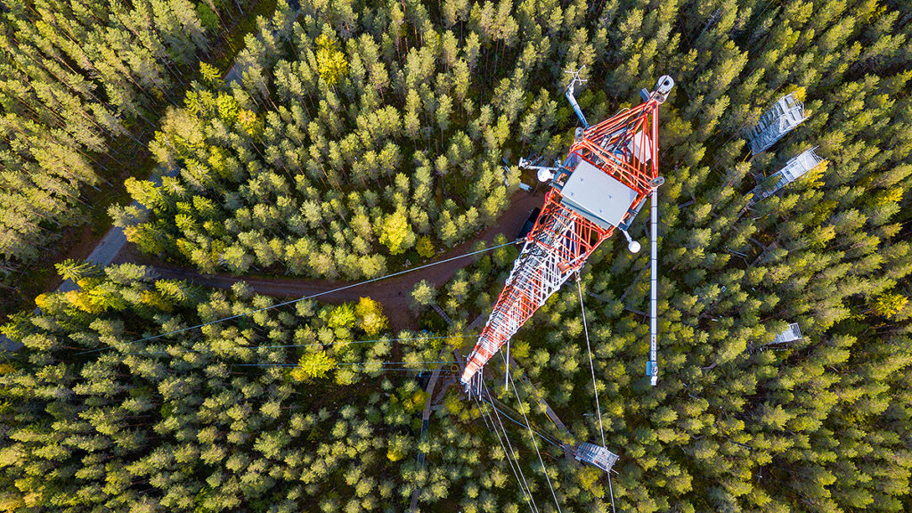
The partnership started with Oldham visiting a 175-foot-tall (53-meter-tall) FLUXNET tower near Sisters, Ore., that Still and his team monitor.
At the top of the tower, a PhenoCam takes photos of the surrounding Deschutes National Forest every half hour. Still uses data from these images to examine how the greenness of the canopy changes over time because such changes can provide information about fluxes in carbon, water, and energy.
“I learned more about what Chris uses the PhenoCam for and got superexcited about the fact that Chris is using color data to understand forests,” Oldham said. “I thought that that was a really beautiful point of overlap for us as a scientist and an artist, to think about color and forests and what we can learn from color as a scientific tool.”
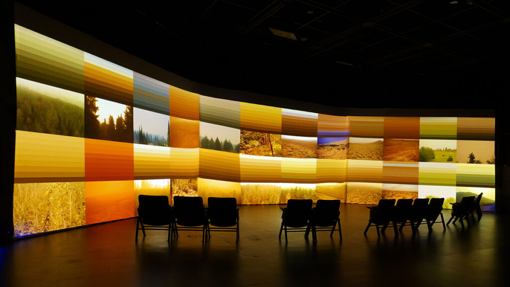
The pair created two pieces. 18//Flux shows how the colors and light from one PhenoCam site changed from 4 a.m. to 9 p.m. throughout the year for 13 years. Each frame is divided into 13 strips, with each strip representing 1 hour of the monitoring period.
The two had conversations throughout the duration of the project about the growing role of wildfires in the area. In fact, one of the FLUXNET towers they were using in the project burned down.
Their conversations led to September: Orange, a three-channel video showing footage from 24 different PhenoCams in the northwestern United States and Canada. When all of the landscapes are the same shade, the video briefly pauses. In September, when wildfires sweep through Cascadia, orange becomes the dominant color. The piece is accompanied by field recordings from Oregon forests and sonified canopy greenness data.
“I think the installation was a wild success, and I had a lot of people tell me how much they enjoyed it and appreciated it,” Still said. “Most people don’t respond to a 2D graph of data…whereas I think almost everyone responds to images, and photographs are really meaningful to people. So I think that is a really brilliant way to draw people into the science.”
—Emily Gardner (@emfurd.bsky.social), Associate Editor


The space industry is surging. In coming years, nearly 10,000 spacecraft are slated to launch into low-Earth orbit for a variety of purposes, such as global surveillance, space tourism, and satellite “megaconstellations” providing internet service.
Rocket engine exhaust, as well as the burnup of inactive satellites and rocket parts reentering Earth’s atmosphere, releases a suite of pollutants. These chemicals have long been considered to pose little threat to our climate, given the historically small size of the space industry. Now, the sector’s rapid growth will send its emissions skyrocketing—but scientists don’t yet have a clear picture of the environmental ramifications.
An analysis by Vliex et al. of rockets launched in 2022 revealed that spaceflight depletes the ozone layer and contributes to global warming, with a significant portion of this ozone loss attributable to nitrogen oxide emissions released by objects reentering Earth’s atmosphere.
The researchers calculated emissions from all 186 rockets launched in 2022, as well as all 472 objects—with a combined total mass of nearly 5,000 tons—that reentered the atmosphere that year. They conducted computational simulations of each launch’s trajectory and emissions at various altitudes up to 100 kilometers, and they calculated emissions released by object reentry. They also accounted for the effects of chemical reactions that occur in rocket exhaust plumes, which alter emissions’ chemical composition.
Incorporation of the calculated emissions into GEOS-Chem, a computational model of atmospheric chemistry, revealed their ozone-depleting and Earth-warming effects, with reentry emissions identified as playing a key role in ozone depletion. The researchers found that accounting for plume reactions reduced the estimated effects of spaceflight emissions, highlighting the value of considering plume chemistry in future assessments.
The analysis also underscored the varying effects of different rocket fuel types. Solid-state fuels, used recently in rocket boosters for NASA’s Artemis II mission to return astronauts to the Moon, appeared to cause the greatest amount of ozone depletion relative to propellant mass, while rocket-grade kerosene caused the greatest amount of warming.
On the basis of their findings, the researchers call for further research into reentry emissions and rocket plume chemistry as the space industry continues to expand and evolve. (Earth’s Future, https://doi.org/10.1029/2025EF007795, 2026)
—Sarah Stanley, Science Writer

hayksenekerimyan posted a photo:
![]()
Where Silence Learns to Speak.
Some places don’t ask you to move on — they simply ask you to stay still for a while.
Black-and-white moments have a way of turning silence into memory.
![]()
