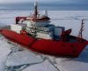
Brazil is expanding its Antarctica presence and activities with the introduction of a new polar vessel currently under construction in the county. The vessel “Almirante Saldanha” is considered an operational and scientific leap for the Brazilian Navy in the context of the strategic development of the Brazilian Antarctic Program.
Brazil is expanding its Antarctica presence and activities with the introduction of a new polar vessel currently under construction in the county. The vessel “Almirante Saldanha” is considered an operational and scientific leap for the Brazilian Navy in the context of the strategic development of the Brazilian Antarctic Program.
Research & Developments is a blog for brief updates that provide context for the flurry of news that impacts science and scientists today.
Human-driven climate change is driving the rise of sea levels, worsening flood conditions and threatening coastal communities around the world. Not only is sea level rising, but it’s rising faster every year. Understanding the degree to which different processes contribute to sea level, known as the sea level budget, can help scientists better pre
Research & Developments is a blog for brief updates that provide context for the flurry of news that impacts science and scientists today.
Human-driven climate change is driving the rise of sea levels, worsening flood conditions and threatening coastal communities around the world. Not only is sea level rising, but it’s rising faster every year. Understanding the degree to which different processes contribute to sea level, known as the sea level budget, can help scientists better predict where and how quickly sea level will rise under potential climate futures.
But for several decades there has been a “budget gap” between measurements of sea level change and the total estimated contributions from glaciers, polar ice, land storage, and oceans expanding as they heat up (thermospheric expansion). Research published today in Science Advances has helped close that budget gap by incorporating more recent sea level observations, reconciling measurements taken by different instruments, and including recent community estimates of sea level rise and its components.
The new analysis breaks down the drivers of sea level rise from 1960 to 2023. The team found that the largest contributor is heat-driven expansion of seawater, responsible for 43% of sea level rise since 1960. Melting ice contributed the next largest amount of sea level rise: 27% came from mountain glaciers, while 15% came from the Greenland Ice Sheet and 12% from the Antarctic Ice Sheet. Lastly, sea level rose 3% as land reduced its capacity to store water.
Since 1960, 43% of global sea level rise can be attributed to thermal expansion of water, just 3% to a reduction in land water storage, and the remainder from melting ice and glaciers. Credit: Zheng et al., Science Advances (2026)
“For years, there has been a frustrating gap between how much the oceans were observed to be rising and how much we could explain from the individual causes,” John Abraham, an engineer at the University of St. Thomas in St Paul, Minn., and a coauthor on the new research, said in a press release. “This work shows that, with better instruments, processes, and smarter analysis, this knowledge gap can be closed. We can explain sea level rise with greater confidence.”
The researchers also calculated the rate at which sea level has risen since 1960 and how each component factored in. They found that the rate of sea level rise has recently doubled: It was 2 millimeters per year averaged over 1960–2023 and 4 millimeters per year averaged over just 2005–2023. The strongest driver of that doubling is ocean warming, responsible for 41% of the accelerating rate of sea level rise, followed by reduced land water storage (21%).
In the past, glacial melt was the largest contributor to sea level rise before it was overtaken by thermospheric ocean expansion overtook (left). The rate of sea level rise has been speeding up since about 1980, also driven by thermospheric ocean expansion (right). Credit: Zheng et al., Science Advances (2026)
This research demonstrates the importance of maintaining detailed records of sea level rise, collecting new measurements, and not backing away from global change research. With better data on which processes contribute to sea level rise and its acceleration, policymakers and local communities can create informed mitigation strategies that account for future rise.
These updates are made possible through information from the scientific community. Do you have a story about science or scientists? Send us a tip at eos@agu.org.
World food commodity prices rose in March for the second month in a row, due largely to higher energy prices linked to the conflict escalation in the Near East, according to the latest benchmark measure released by the Food and Agriculture Organization of the United Nations (FAO).
World food commodity prices rose in March for the second month in a row, due largely to higher energy prices linked to the conflict escalation in the Near East, according to the latest benchmark measure released by the Food and Agriculture Organization of the United Nations (FAO).
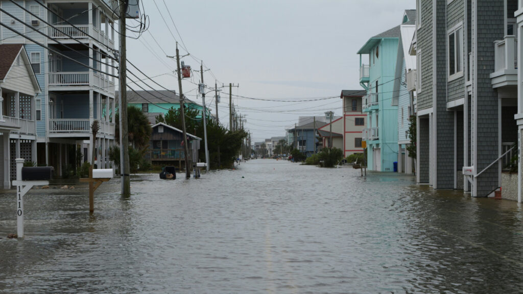
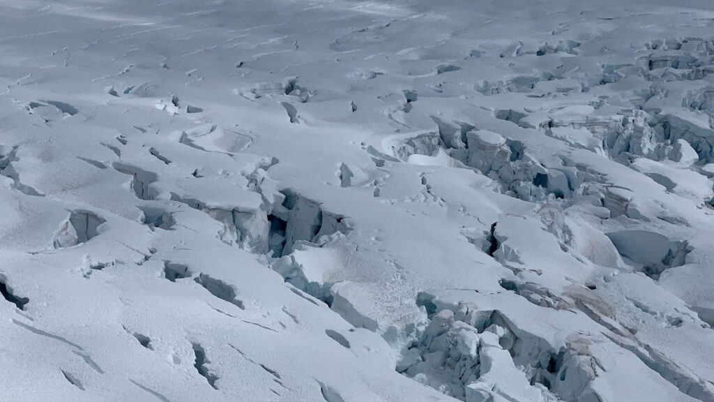
The retreat of glaciers and ice sheets is expected to have widespread impacts on communities around the world because of its effect on sea levels. Already, the global average sea level is more than 10 centimeters higher than it was just 3 decades ago; and the rate of rise is increasing, contributing to increased storm surges and flooding, lost infrastructure and community lands, and more.
Recent reports on the instability of Antarctica’s Thwaites Glacier, for example, have focused attention
The retreat of glaciers and ice sheets is expected to have widespread impacts on communities around the world because of its effect on sea levels. Already, the global average sea level is more than 10 centimeters higher than it was just 3 decades ago; and the rate of rise is increasing, contributing to increased storm surges and flooding, lost infrastructure and community lands, and more.
Recent reports on the instability of Antarctica’s Thwaites Glacier, for example, have focused attention on how accelerating ice flow can lead to ice sheet collapse and rising sea levels.
Earth’s ice sheets accumulate ice through snowfall and lose mass through a mix of surface ablation, iceberg calving, and melting at their interface with the ocean. Glacial ice flows under its own weight, and the rate at which it flows to coastal areas is a primary control on ice sheet mass loss.
Flow rates depend on how much resistance an ice sheet encounters at its interface with the ground (e.g., whether it is frozen to its substrate) and on its effective viscosity, a measure of how strongly it resists deformation. The viscosity of ice, in turn, varies based on properties including temperature, crystal size and orientation, and impurity content.
Some properties within and beneath ice sheets that affect how they flow are anisotropic, meaning they vary by direction. For example, roughness in some directions at the ice bed can facilitate ice sliding more effectively than roughness in other directions, similar to the way a properly oriented corrugated metal roof allows snow to slide off. Several forms of anisotropy within ice also affect how ice flows from land to ocean (Figure 1).
Fig. 1. Anisotropy in glaciers and ice sheets has various sources, including from ice fabric and other properties within the ice (englacial) or at the ice-bed interface. Many forms of anisotropy in glacial ice can be measured with radar. Credit: Adapted from Hills et al., 2025, https://doi.org/10.1029/2024RG000842, CC BY 4.0
Measuring anisotropic properties is key to better understanding how quickly changes at the edges of the Greenland and Antarctic ice sheets will lead to sea level rise. Recent advances in ice-penetrating radar technology and in processing radar data are revolutionizing how we observe directionally varying ice sheet properties, paving the way for projections of mass changes that account for previously neglected processes.
Crystal Fabric: Memory and Modulator of Ice Flow
Fabric, the orientation of crystals composing ice, is the best studied and arguably most important of anisotropic ice sheet properties. As ice deforms, for example, by stretching horizontally as it flows toward the coast, its millimeter-scale crystals are reoriented (Figure 1).
Fabric thus contains a memory of past flow. Simultaneously, fabric influences flow because ice crystals are about 3 orders of magnitude easier to shear in some directions than others—similar to how stacked playing cards slide easily against each other when held along their edges but resist motion when pinched top to bottom.
Over the past 20 years, radar polarimetry has matured into a quicker and easier alternative means for inferring fabric.
The potential importance of fabric on large-scale ice flow has long been recognized, but a shortage of observations has made it difficult to quantify and validate its effect in ice sheet models. Until recently, fabric could be measured only directly in ice cores or inferred through seismic soundings. These methods provide highly detailed information about how fabric develops but are expensive, logistically taxing, and provide information only about sparse point locations.
Over the past 20 years, though, radar polarimetry has matured into a quicker and easier alternative means for inferring fabric, enabling observations at the scale of entire glaciers and providing new constraints on how fabric influences ice sheet flow.
How Radar Reveals Fabric
Ice-penetrating radar instruments emit electromagnetic energy as radio frequency waves. These waves reflect off interfaces within and beneath glacial ice, including transitions in ice chemistry and the contact surface between the ice sheet and the ground or water below. The properties of the reflected waves are then measured when they return to the radar. Just as fabric leads to anisotropic ice deformation, it also introduces directional dependence in the measured electrical properties.
The speed of a radar wave through an ice crystal is approximately 1% faster if the wave is polarized across the crystal’s principal (c) axis rather than aligned with it. Though small, this difference can compound enough that it causes measurable changes in returned radar signals.
In a typical radar survey over anisotropic ice, waves with different polarizations travel at slightly different speeds (Figure 2). The times that return signals arrive back at the receiver thus vary directionally, a difference that can be identified using polarimetric radars that transmit and receive radio waves at multiple orientations.
Fig. 2. Propagation of polarized radio waves through anisotropic ice reveals structural variations with depth because waves aligned across the prevailing ice fabric (represented by the ball, in which darker shading indicates a greater concentration of c axes) travel faster than waves aligned with the fabric. The phase delay increases as the effect of the anisotropy accumulates with depth. Credit: Adapted from Hills et al., 2025, https://doi.org/10.1029/2024RG000842, CC BY 4.0
Fabric’s effect on radar signal travel times accumulates through an ice column, so it is more prominent in thicker ice with stronger horizontal fabric (i.e., the ice crystals are more consistently aligned). In such cases, differences in travel times between polarizations can be measured even by standard radars.
When fabric is weaker or ice is thinner, the offset is smaller and detectable only by systems that can identify the phases of radar returns—that is, the exact positions of the returned waves in their oscillation cycle. Even small wave speed differences from weak fabrics accumulate into measurable phase shifts between polarizations, which can be used to determine the consistency of crystal alignment and the predominant crystal orientation.
Small differences in fabric through an ice column can also change the strength, or amplitude, of returned signals. This amplitude difference offers an independent way to identify fabric orientation and its depth variation.
Polarimetric radar has been widely applied in cryospheric science in recent years largely due to the advent of low-cost systems that can measure signal phases. For example, the popular Autonomous phase-sensitive Radio Echo Sounder (ApRES) is a lightweight, ground-based system that can be used to infer ice fabric at single points down to 2 kilometers deep. In the past decade, polarimetric ApRES systems have revealed ice flow histories, including changes in flow directions, of key glaciers over the past few millennia. These measurements offer windows into how ice sheets responded to previous climate variations.
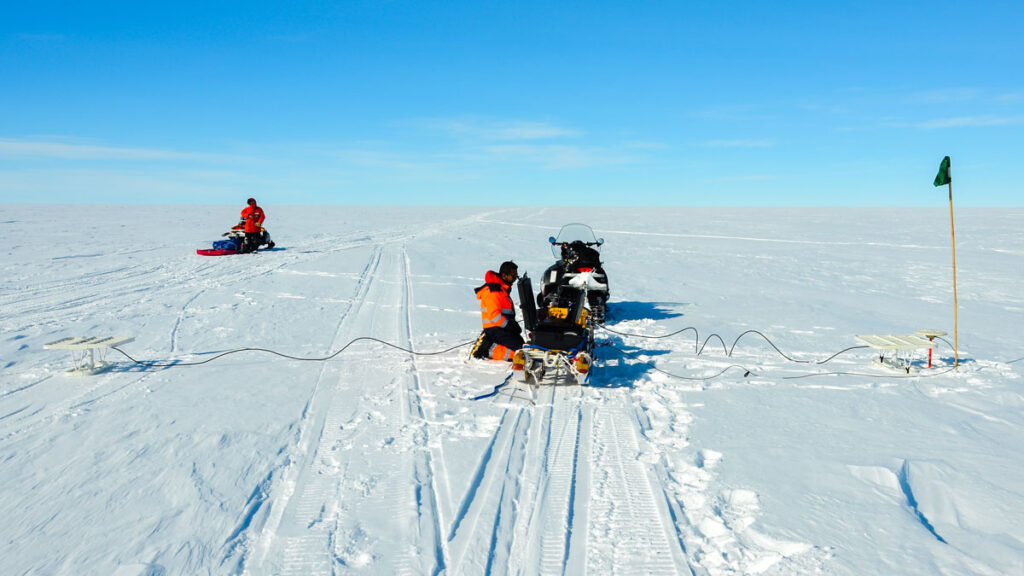
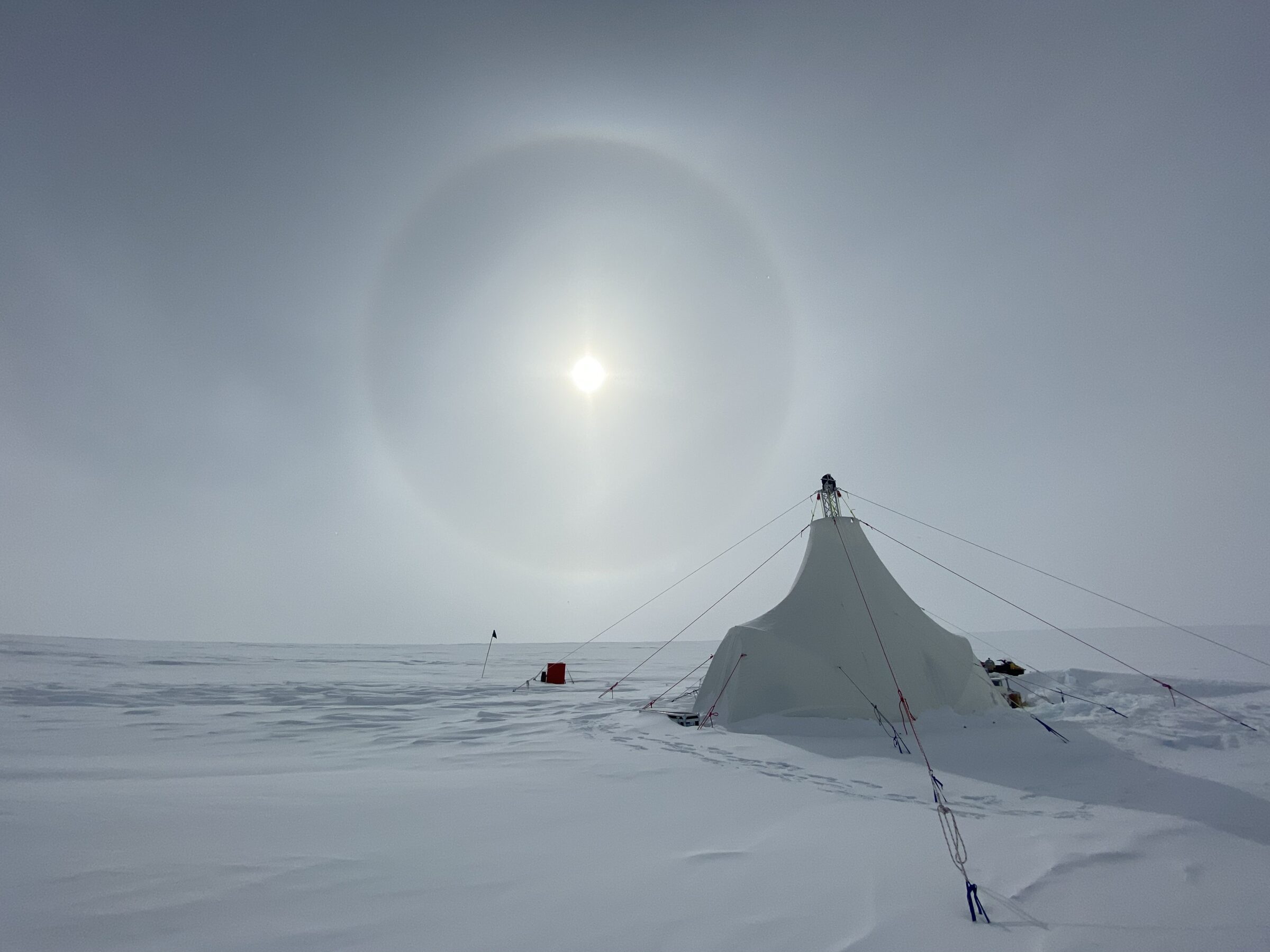
A mobile, quad-polarimetric radar is dragged by snowmobile over the surface of Müller Ice Cap on Axel Heiberg Island in Nunavut, Canada, in May 2023. Credit: David Lilien
The next generation of polarimetric radars go beyond one-point-at-a-time stationary soundings, offering full polarimetry capabilities on moving platforms. These systems may soon allow scientists to map directional ice properties at the scale of entire ice sheets.
Insights into Fast-Flowing Ice Fabric
The growing number of radar studies conducted near sites where ice cores have been collected, which allow fabric to be investigated up close, has provided validation and bolstered confidence that fabric can be inferred accurately from its effects on radar. Researchers now infer fabric from radar in more dynamic areas, such as Thwaites Glacier, Whillans Ice Stream, and the Northeast Greenland Ice Stream (NEGIS), where ice fabrics change over short spatial scales and where drilling ice cores is logistically difficult. Airborne radar surveys are particularly effective in these settings because they can efficiently map fabric variations across large, fast-moving areas.
Observations of strong fabrics in fast-flowing regions suggest that fabric is an important control on ice viscosity, although its implications for ice flow are just beginning to be explored. For example, at Rutford Ice Stream in Antarctica, ApRES data indicate that fabric causes sharp changes in viscosity in different directions with depth, a complexity not captured by current ice flow models.
A combination of airborne and ground-based radar shows that the fabric of the NEGIS varies substantially across the ice stream, which facilitates horizontal shear that allows faster and more cohesive flow in the middle of the ice stream while simultaneously stiffening this ice against along-flow stretching. These viscosity variations may alter how quickly coastal changes, such as increased melt due to climate warming, influence inland ice flow.
Scientists have studied ice sheet mass balance at glacier-mounted stations along the renowned “K-transect” near Kangerlussuaq in southwestern Greenland since the early 1990s. This image shows a view up the transect in April 2025. Polarimetric radar offers another tool with which to study ice flow here and at other locations on the ice sheets. Credit: Tamara Gerber
The emerging consensus from radar observations and recent progress in fabric modeling is that ice fabric can soften ice stream shear margins by a factor of 10. In other words, the fabric tends to develop in a way that greatly reduces the ice’s effective viscosity at lateral boundaries between fast-flowing and slower-flowing ice, which enables the ice to deform more easily at the margins. The agreement between observations and process-scale modeling highlights fabric as a major, but largely ignored, control on ice flow that may affect estimates of how ice dynamics will contribute to future sea level rise.
Beyond Fabric
Most polarimetric radar studies so far have focused on fabric, but other ice characteristics can cause directional effects too. For instance, bubbles trapped in ice have dramatically different properties than ice itself. Ice deformation can bring bubbles into alignment, such that they affect radar waves differently in different directions.
Likewise, ice at its melting point can contain liquid water along boundaries between crystals, and if those pockets of water are aligned in one direction, they can also affect radar returns. Each of these properties has important influences on ice flow, but their implications are yet to be explored.
Another source of anisotropy is the bottom boundary of the ice sheet. This interface can be rougher in some directions than others, though the roughness is typically aligned with the prevailing ice flow direction or the direction of meltwater trapped within the ice.
Polarimetric radar can measure directionally dependent properties of ice sheet bases at a finer scale than radar profiling can. Such work is leading to new insights into glacier geomorphology, interactions of ice shelf bottoms with the underlying ocean, and how ice slides over substrate surfaces. Rates and extents of sub-ice-shelf melt and basal sliding are widely recognized as key controls on the future of the ice sheets.
Expanding Horizons: Large-Scale and Planetary Applications
Radar polarimetry has already transformed our understanding of ice fabric, revealing much about how crystal alignment modulates the flow of Earth’s ice sheets and filling critical gaps between the handful of direct measurements from ice cores. As polarimetric techniques mature, their applications are expanding.
Researchers are moving from studying isolated profiles of ice fabric to mapping it across whole basins, a key shift for validating bespoke models of fabric and its effects on flow. These models are also rapidly developing to include additional physical processes (e.g., migration recrystallization) and key simplifications (e.g., reducing directionally varying viscosity to a single number) that allow them to interface more easily with—and be incorporated into—large-scale models used for projecting sea level rise.
Techniques pioneered for measuring ice on Earth may also prove useful elsewhere in the solar system.
Techniques pioneered for measuring ice on Earth may also prove useful elsewhere in the solar system. Orbital radar sounders have already probed Mars’s ice masses, and the icy shell of Jupiter’s moon Europa will soon be surveyed by single-polarization radars aboard NASA’s Europa Clipper and the European Space Agency’s Jupiter Icy Moons Explorer (JUICE). These radars might be useful for polarimetry at some locations on Europa, which could reveal past and present motion of ice features and answer fundamental questions about the moon. Whether Europa’s shell flows, for example, may be key to whether its subsurface ocean can harbor life.
As polarimetric radar systems become routine tools for glaciologists and as similar instruments begin operating on spacecraft exploring icy worlds, a technique once limited to a few isolated core sites on Earth could be poised to transform our understanding of ice across the solar system.
Author Information
David Lilien (dlilien@iu.edu), Indiana University Bloomington; T. J. Young, University of St Andrews, Fife, Scotland; Benjamin Hills, Colorado School of Mines, Golden; Tamara Gerber, Université de Lausanne, Lausanne, Switzerland; and Matthew Siegfried, Colorado School of Mines, Golden
Citation: Lilien, D., T. J. Young, B. Hills, T. Gerber, and M. Siegfried (2026), New directions in mapping ice sheet fabrics and flow, Eos, 107, https://doi.org/10.1029/2026EO260154. Published on 14 May 2026.
Editors’ Highlights are summaries of recent papers by AGU’s journal editors.
Source: Journal of Geophysical Research: Earth Surface
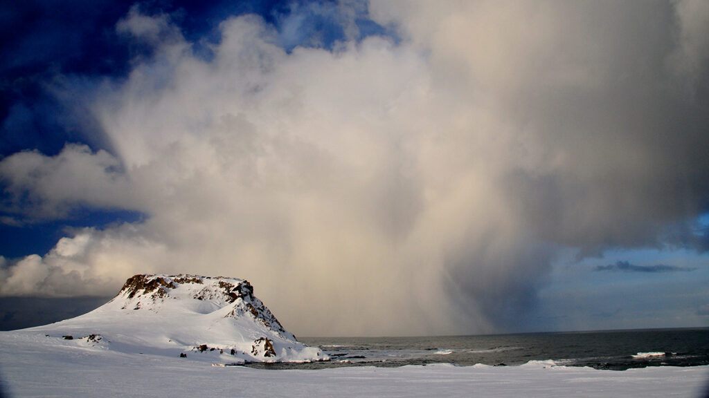
Antarctica’s snow and ice surfaces play a key role in how the continent exchanges heat and moisture with the atmosphere. A key property controlling this exchange is aerodynamic roughness length (zo), which measures how “bumpy” the surface is. Rougher surfaces, such as snow sastrugi (wind-formed ridges and grooves), interact more strongly with the air above, a
Source: Journal of Geophysical Research: Earth Surface
Antarctica’s snow and ice surfaces play a key role in how the continent exchanges heat and moisture with the atmosphere. A key property controlling this exchange is aerodynamic roughness length (zo), which measures how “bumpy” the surface is. Rougher surfaces, such as snow sastrugi (wind-formed ridges and grooves), interact more strongly with the air above, affecting snow movement, melting, and local environmental conditions. Despite its importance, zo is often treated as a single, constant value over large areas in Earth system models because it is difficult to measure.
Zheng et al. [2026] use a multi-temporal Unmanned Aerial Vehicle (UAV) oblique photogrammetry to map fine scale zo variability at Qinling Station in East Antarctica. The results show that zo can vary substantially depending on surface type, measurement scale, model choice, and meteorological conditions. The complex response of surface microtopography to meteorological events is a noteworthy new finding. For example, in snow sastrugi areas, zo can vary by an order of magnitude over time, increasing after snowfall and decreasing under strong winds. These findings highlight that capturing fine-scale surface roughness is essential for accurately modeling snow–atmosphere interactions in Antarctica and could help improve current weather and climate models for polar regions.
Citation: Zheng, Z., Zheng, L., Wang, K., Clow, G. D., & Cheng, X. (2026). UAV oblique imagery reveals order-of-magnitude changes in snow aerodynamic roughness length under shifting meteorological regimes at Qinling Station, East Antarctica. Journal of Geophysical Research: Earth Surface, 131, e2025JF008781. https://doi.org/10.1029/2025JF008781
Source: AGU Advances
Models of glacial flow and retreat rely on estimates of glacial ice viscosity, the measure of the ice’s resistance to flow.
Ice viscosity is dependent on the stress applied to the glacier. Most ice sheet models use a standard equation to model ice flow that includes the variable n, called the stress exponent. A larger value of n means ice viscosity is more sensitive to changes in stress. For decades, glaciologists have, almost exclusively, used an assumed n value of 3
Models of glacial flow and retreat rely on estimates of glacial ice viscosity, the measure of the ice’s resistance to flow.
Ice viscosity is dependent on the stress applied to the glacier. Most ice sheet models use a standard equation to model ice flow that includes the variable n, called the stress exponent. A larger value of n means ice viscosity is more sensitive to changes in stress. For decades, glaciologists have, almost exclusively, used an assumed n value of 3 in the models they use to predict ice flow.
However, through recent experiments and observations, researchers have found that an n value of 4 may actually better represent the conditions of Earth’s ice sheets and glaciers.
Martin et al. created a model representation of the fast-retreating Pine Island Glacier in West Antarctica. The ice sheet in their model had a true n value of 4, but they ran model projections using both n = 4 and n = 3. That allowed them to observe how their model would incorrectly predict glacial flow and resulting sea level change, given an incorrect n value.
The researchers modeled glacial retreat for 100 years under both equations with two different glacial melting scenarios. They then modeled glacial recovery for another 300 years. Under a moderate scenario, the n = 3 model underestimated glacial retreat by 18% and sea level change contributions by 21%. Under an extreme melting scenario, the model underestimated sea level contributions by 35%.
Notably, those disparities in glacial retreat and sea level change contribution predictions increased more than would be expected between the two scenarios, potentially increasing the level of uncertainty in current projections of sea level change. The researchers also suggest that incorrect n values may be mistakenly attributed to other physical processes in current ice sheet models.
The results could have far-reaching implications for predictions of future glacial melt and may prompt investigations into its effects on sea level, the authors say. (AGU Advances, https://doi.org/10.1029/2025AV001946, 2026)
—Madeline Reinsel, Science Writer
Citation: Reinsel, M. (2026), Glaciers may flow into the ocean more quickly than we think, Eos, 107, https://doi.org/10.1029/2026EO260107. Published on 14 April 2026.
Source: Geophysical Research Letters
Atmospheric rivers act like “rivers in the sky,” shuttling intense bands of warm, heavy moisture from lower to higher latitudes. When an atmospheric river encounters cold air or mountainous terrain, the moisture it carries condenses and falls as heavy rain or snow. In Antarctica, the arrival of an atmospheric river can help build surface ice mass. Much of Antarctica is very dry; an atmospheric river can bring the moisture needed to potentially offset some
Atmospheric rivers act like “rivers in the sky,” shuttling intense bands of warm, heavy moisture from lower to higher latitudes. When an atmospheric river encounters cold air or mountainous terrain, the moisture it carries condenses and falls as heavy rain or snow. In Antarctica, the arrival of an atmospheric river can help build surface ice mass. Much of Antarctica is very dry; an atmospheric river can bring the moisture needed to potentially offset some ice loss.
Antarctica’s varied topography and dry conditions have made detecting atmospheric rivers over the continent challenging. Previous efforts to do so have suggested that atmospheric rivers contribute up to 30% of Antarctica’s total annual precipitation, but these methods may not be capturing the full picture of atmospheric river activity.
Takahashi et al. developed a new 3D atmospheric river detection algorithm to better capture how atmospheric rivers affect Antarctica’s complex terrain. Previous methods have mostly been 2D, meaning they do not accurately account for the vertical variations within an atmospheric river.
To evaluate the algorithm, the researchers applied it to two datasets: (1) daily snowfall totals measured during the 44th Japanese Antarctic Research Expedition (JARE44) at Dome Fuji from February 2003 to January 2004 and (2) the ERA5 (European Centre for Medium-Range Weather Forecasts atmospheric reanalysis) dataset of daily weather patterns and conditions in Antarctica from 1979 to 2023.
The results of the study’s new algorithm showed 16 significant snowfall events during the JARE44 expedition, all of which were not detected by the older 2D method. The new 3D method identified 17 days of atmospheric river activity, which corresponded with 10 heavy snowfall events and accounted for approximately 40% of the total precipitation. Between 1979 and 2023, atmospheric rivers occurred about 10% of the time yet contributed 30%–60% of total precipitation in the Antarctic interior.
The 3D method in the new study suggests that atmospheric river events contribute a greater proportion of total snowfall than previously thought—between 30% and 90%, depending on the Antarctic region. The researchers also suggest that long-term changes in Antarctic snowfall are closely linked with the changes in atmospheric river activity. This connection is especially apparent in East Antarctica, where the link between snowfall increases and atmospheric rivers had not yet been clearly identified in previous studies. (Geophysical Research Letters, https://doi.org/10.1029/2025GL120986, 2026)
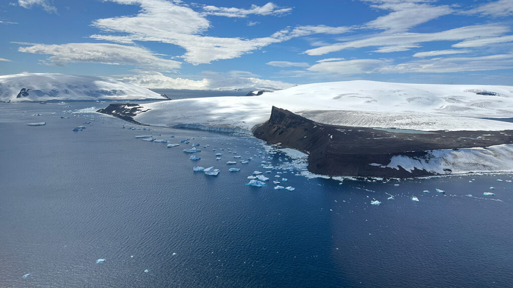
A critical ocean current that regulates Antarctica’s climate may have formed only once continents separated and winds aligned with new ocean passageways, according to a new study published in the Proceedings of the National Academy of Sciences of the United States of America.
Today, the Antarctic Circumpolar Current transports more than 100 times as much water as all of Earth’s rivers combined and, critically, insulates the Antarctic Ice Sheet from heat at lower latitudes. A clear picture of
Today, the Antarctic Circumpolar Current transports more than 100 times as much water as all of Earth’s rivers combined and, critically, insulates the Antarctic Ice Sheet from heat at lower latitudes. A clear picture of the origins of this current can help scientists further understand the relationships between contemporary ocean dynamics, the global climate, and ice formation in Antarctica.
“It’s very interesting to learn more about this current, how it developed, and what role it played in the climate change that was happening at that time,” said Hanna Knahl, a paleoclimatologist and doctoral student at the Alfred-Wegener-Institut in Germany and lead author of the new study.
The Birth of a Current
About 34 million years ago, Earth was undergoing a climatic shift, now known as the Eocene-Oligocene transition, during which atmospheric carbon dioxide decreased and the planet cooled.
Earth’s tectonic plates in the Southern Ocean moved away from each other, opening and deepening bodies of water such as the Tasmanian Gateway and the Drake Passage, which separate Antarctica, Australia, and South America.
For years, scientists hypothesized that the alignment of these newly formed waterways, along with westerly winds, could have channeled ocean water and spurred the formation of the Antarctic Circumpolar Current.
“The exact position of the westerly winds and their relative position to the [ocean] gateways have to click together.”
To test that hypothesis, Knahl and her colleagues simulated conditions of the early Oligocene Southern Ocean with a coupled model that included ocean dynamics, atmosphere and wind patterns, temperatures, ice sheet growth, and precipitation. The research team compared these simulations to data from actual Antarctic sediment cores and scans of the ocean floor.
Results confirmed that westerly winds were necessary for the Antarctic Circumpolar Current to form.
“The exact position of the westerly winds and their relative position to the [ocean] gateways have to click together,” Knahl said.
Joanne Whittaker, a marine geophysicist at the University of Tasmania who was not involved in the new study, was a coauthor of a 2015 study that proposed westerly wind alignment played a role in the formation of the current. Knahl’s study presents a more sophisticated model of the early Oligocene Southern Ocean and is a great next step in the investigation of the current’s origins, Whittaker said.
“They did a really nice job of taking a range of different people’s work and linking it all together,” she said.
Oligocene Understandings
“If you can have a model that works in the past, it’s going to give you confidence that it’s going to work for the future, as well.”
Scientists often use Earth’s past behavior to better understand how Earth systems may behave in the present or future. “If you can have a model that works in the past,” Whittaker explained, “it’s going to give you confidence that it’s going to work for the future, as well.”
The Eocene-Oligocene transition is a key to understanding the relationship between atmospheric carbon, ocean dynamics, and the glaciation of Antarctica, Whittaker said. Knowing how the current’s behavior affected carbon uptake millions of years ago helps scientists model how the present current’s behavior might also affect atmospheric carbon.
In addition to carbon uptake, the new research hints at how changes in westerly winds may influence the advance and retreat of the Antarctic Ice Sheet. Some modeling and proxy data indicate the westerly winds that spurred the Antarctic Circumpolar Current’s formation 34 million years ago have shifted in the past century and may continue to shift in the future. Understanding the role these winds initially played in the current’s development may shed light on the current’s present ability to guard the Antarctic Ice Sheet from warmer air masses.
There are still Oligocene patterns that require more research to sort out, though. For example, modeling in the new study showed interesting asymmetries in the timing of the development of different parts of the Antarctic Circumpolar Current, Knahl said. Scientists know from proxy data and modeling that similar asymmetry exists in the history of the Antarctic Ice Sheet; the ice sheet in East Antarctica began to form about 7 million years before the ice sheet began to form in West Antarctica.
“It could be interesting to see if there’s a connection between the asymmetries that we see here,” Knahl said. “Are they linked, or were they more or less independent?”
Citation: van Deelen, G. (2026), Widening channels and westerly winds together formed Earth’s strongest current, Eos, 107, https://doi.org/10.1029/2026EO260126. Published on 24 April 2026.
Exclusive A vast area of the Bellingshausen Sea should be covered by sea ice by now, with one expert calling the loss of ice ‘depressing’Antarctica’s west coast is missing an area of winter sea ice the size of France, sparking concerns for threatened penguins other marine life and global sea levels.One expert said the loss of ice in the Bellingshausen Sea was “depressing” and the failure of ice to form could have intensified a heatwave over the continent’s peninsula last week that saw daytime te
Exclusive A vast area of the Bellingshausen Sea should be covered by sea ice by now, with one expert calling the loss of ice ‘depressing’
Antarctica’s west coast is missing an area of winter sea ice the size of France, sparking concerns for threatened penguins other marine life and global sea levels.
One expert said the loss of ice in the Bellingshausen Sea was “depressing” and the failure of ice to form could have intensified a heatwave over the continent’s peninsula last week that saw daytime temperatures peak at 15.4C which is more than 20C above average.
Seeking Solutions to PFAS Pollution
Chemical Companies Are Churning Out New PFAS. Where in the World Are They Ending Up?
The Persistence of PFAS
A Peculiar Polymer Paired with Sunlight Could Remove PFAS
Tracing the Path of PFAS Across Antarctica
Pollution Is Rampant. We Might As Well Make Use of It.
Per- and polyfluoroalkyl substances (or PFAS) have been widely used in thousands of common nonstick, waterproof, or stain-resistant products since the 1950s. These “forever c
Per- and polyfluoroalkyl substances (or PFAS) have been widely used in thousands of common nonstick, waterproof, or stain-resistant products since the 1950s. These “forever chemicals” do not break down easily: PFAS make their way into the air, soil, and water, as well as into human and animal bloodstreams and to some of Earth’s most pristine environments. They have been detected even in Antarctica, despite its reputation as a relatively untouched landscape far from the types of products—fast-food wrappers, firefighting foam, nonstick cookware—that contain PFAS.
Research into how PFAS arrive in Antarctica is limited, and most tends to focus on the continent’s coasts, rather than its interior. A new study published in Science Advances aimed to fill some of these gaps by examining PFAS accumulation across a 1,200-kilometer stretch of Antarctica, from the snow pits of Zhongshan Station in East Antarctica to the 4,093-meter peak of Dome A. By examining layers of snow collected from the coast to the interior, researchers sought to better track and understand how PFAS levels vary by location and how these forever chemicals have been able to travel long distances through the upper atmosphere to be deposited in remote regions.
“For substances to get there, they have to be able to transport long distances,” said Ian Cousins, a chemist at Stockholm University and one of the study’s authors. “We know PFAS are very persistent, so that helps. By looking at the patterns of the PFAS contamination in the samples, it gives us clues as to how they’re transported.”
PFAS Arrive by Air and by Sea
Along the 1,200-kilometer route, researchers from the Chinese Academy of Sciences collected 39 snow samples at 30-kilometer intervals, scraping the first few centimeters of snow from the surface to analyze for traces of PFAS.
Zhongshan Station sits near Prydz Bay, and there, researchers collected snow from a 1-meter-deep pit, with samples taken every 5 centimeters. At Dome A, the summit of the East Antarctic Ice Sheet, samples were collected at 10-centimeter intervals from another snow pit; this one was 3 meters deep, providing information about the past several decades of PFAS use.
“It’s quite interesting that we see the historical production record of PFAS in this pit on the top of this mountain in Antarctica,” said Cousins.
PFAS pollution arrives in Antarctica in two ways: via upper atmospheric transport and sea spray. Some PFAS are formed in the atmosphere when volatile precursor chemicals like fluorotelomer alcohols used in textile and paper products break down through reactions with sunlight and oxidants into more stable compounds. The resulting PFAS are later deposited into the snow and ice through precipitation.
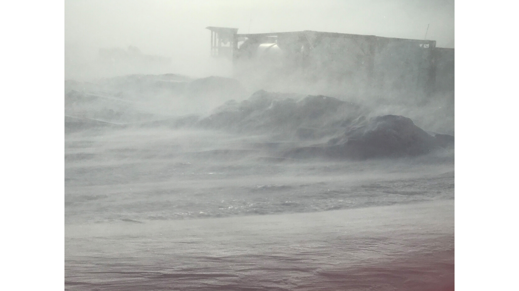
Storm winds near the coast create sea spray. “When you have waves, it makes bubbles in the ocean. When the bubbles burst, these sea spray aerosols can be super enriched with PFAS. This has been shown to be a very important transport route,” Cousins said.
To distinguish between sources, researchers measured sodium in the snow to trace the ocean’s salty influence. Sodium levels decreased farther inland, reflecting the fading influence of sea spray toward the interior of the continent. But surprisingly, PFAS concentrations actually increased moving from the coast into the interior.
“That was kind of a bit counterintuitive to me,” explained Cousins, who said he expected PFAS levels to be highest near the coast. “You see the opposite, actually.”
The inland increase is likely explained by higher snowfall totals in the coastal regions, which lead to PFAS concentrations becoming diluted. Inland, where snowfall is lower, even small amounts of PFAS can result in relatively higher concentrations within snow samples.
Additional factors shape PFAS distribution. PFAS levels are higher at the onset of precipitation events when they are rapidly removed from the air. Temperature inversions, too, can trap chemicals. In coastal areas, PFAS are more influenced by sea spray in the winter, whereas stronger sunlight drives the degradation of atmospheric precursors into PFAS in the summer months.
PFAS Presence at Both Poles
This new study also offers implications for the way that PFAS circulate globally. Though industrial activity in the Northern Hemisphere contributes most heavily to PFAS emissions, large-scale atmospheric circulation allows these compounds to reach polar regions. Rapid transport in the upper troposphere may act as an efficient pathway to shuttle PFAS across both hemispheres before they are deposited in the cold, remote regions at both ends of Earth.
“This completes the global picture with agreeing measurements at both poles, solidifying our understanding of the global distribution and drivers of PFAS contamination.”
Even though PFAS levels are higher in the Arctic, both polar regions show similar trends in PFAS concentrations since the 1990s. “It really matches decades of the same records that have been reported from the Arctic,” said Cora Young, an atmospheric chemist at York University, who was not involved in the new study.
“This completes the global picture with agreeing measurements at both poles, solidifying our understanding of the global distribution and drivers of PFAS contamination. The role of CFC [chlorofluorocarbon] replacements, changes in regulation, all of these things are important in the Northern Hemisphere and also the Southern Hemisphere,” said Young.
Tiny saltwater channels have a big influence on sea ice.
Sea ice typically includes pockets or channels of brine that allow salt water to flow vertically through the ice. When those channels align neatly, they need to make up only about 5% of the ice volume before the water can flow. But in more disordered, granular ice, salt water starts to flow only when the brine channels take up more space—roughly 10% of the ice volume, according to a new study published in Scientific Reports.
“If we’
Tiny saltwater channels have a big influence on sea ice.
Sea ice typically includes pockets or channels of brine that allow salt water to flow vertically through the ice. When those channels align neatly, they need to make up only about 5% of the ice volume before the water can flow. But in more disordered, granular ice, salt water starts to flow only when the brine channels take up more space—roughly 10% of the ice volume, according to a new study published in Scientific Reports.
“If we’re trying to find predictive models about how these ice cores are responding under climate change, it’s going to be necessary to take into account these structural and microstructural conditions.”
This higher threshold could slow the drainage of surface melt ponds, as well as the transport of nutrients to microbial communities inside the ice.
“If we’re trying to find predictive models about how these ice cores are responding under climate change, it’s going to be necessary to take into account these structural and microstructural conditions,” said Stephen Ackley, a sea ice researcher at the University of Texas at San Antonio who was not involved in the study.
Disorderly Constructs
As seawater freezes, it forms a mixture of ice crystals and brine. In calm conditions, the ice slowly grows into long, parallel crystals separated by orderly brine channels. This columnar sea ice is common in the Arctic, and its properties have been widely used in sea ice models.
But in choppy waves or when the ice’s snow-covered surface floods and refreezes, new ice can’t grow into these ordered columns. Instead, it forms small, randomly oriented grains separated by more complex pores containing brine and gases. Called granular ice, this form is more common in Antarctica but is becoming increasingly prevalent in the Arctic as temperatures rise and ice cover thins.
“It’s the sequel we’ve been waiting decades for.”
In 1998, University of Utah mathematician Kenneth Golden established the first estimate of the point at which the brine channels are connected enough to allow water to flow in columnar ice, called the percolation threshold. The new work, also led by Golden, extends a similar analysis to granular sea ice.
“It’s the sequel we’ve been waiting decades for,” said Don Perovich, a sea ice researcher at Dartmouth who was not involved in the new work.
To quantify the percolation threshold for granular ice, Golden and his colleagues collected sea ice samples during two expeditions off the eastern coast of Antarctica in 2007 and 2012. They measured how quickly water moved through the brine channels in the ice. After the 2012 expedition, they also mapped the arrangement of ice crystals within the ice blocks to correlate those permeability measurements with the microscale structure of the ice.
Most climate models are based on the assumption that the microstructure of sea ice is organized into columns, like those in the image on the left. But new research shows that granular ice, as seen on the right, is growing more common in the Arctic, which could affect climate modeling. Credit: Golden et al., 2026, https://doi.org/10.1038/s41598-026-41706-w, CC BY-NC-ND 4.0
The finding that in granular ice, about twice as much of the ice volume needs to be brine for water to flow compared to columnar ice suggests that brine channels within granular ice are much less interconnected.
With the higher threshold, “you have to reassess all these models, anything that relies on fluid flow through sea ice,” if granular ice is present, said Golden. Granular ice will require warmer or saltier conditions to leave enough brine in the ice structure to meet the percolation threshold and allow water to flow vertically.
Researchers extracted blocks of ice in Antarctica with a chainsaw and poured dyed salt water on top. In this way, they observed how quickly the fluid descended through the ice. Credit: Kenneth Golden
For example, the new value could influence models of how meltwater ponds behave atop an underlying ice sheet. If meltwater ponds form above a base of granular sea ice, those ponds will require warmer temperatures before they start draining than melt ponds on columnar ice will.
If these melt ponds remain on the surface longer waiting for those warmer temperatures, they could lower the albedo, or reflectivity, of the ice sheet. That could cause the ice sheet to absorb more heat, leading to a feedback loop that could accelerate melting.
The higher percolation threshold could also affect algae that lives within the ice. Ice algae make up an important food source for krill and crustaceans, which in turn become food for fish, penguins, and whales. Algae rely on water flowing through the ice to deliver nutrients. Because granular ice requires warmer temperatures for that flow to start, it could affect the depth at which algae can live inside the ice, Golden said.
Percolation Consideration
Still, experts say more data are needed to establish percolation thresholds across both Arctic and Antarctic ice. The size of the grains in granular ice can vary substantially at different temperatures, under different formation conditions, and between the poles. Larger grains could lower the percolation threshold, allowing water to flow even when the ice contains much less than 10% brine by volume, said Sønke Maus, a scientist studying ice microstructure at the Norwegian University of Science and Technology who was not involved in the study.
“The data that we have at the moment for the granular sea ice is sparse,” Maus said. “You need a big campaign to collect such data.”
Golden said that in future work he also plans to develop models to compute the electromagnetic properties of both columnar and granular sea ice. Knowing these properties can help scientists determine the thickness and age of an ice sheet from satellite data.
Citation: Ware, S. (2026), Changes in sea ice microstructure could affect climate models, Eos, 107, https://doi.org/10.1029/2026EO260164. Published on 20 May 2026.
Antarctica’s Ross Ice Shelf and the West Antarctic Ice Sheet may have been far smaller during one of Earth’s most recent warm periods, according to a new study.
Antarctica’s Ross Ice Shelf and the West Antarctic Ice Sheet may have been far smaller during one of Earth’s most recent warm periods, according to a new study.