Editors’ Vox is a blog from AGU’s Publications Department.

After 18 years of data collection, quality control, processing, and archiving, the United States Magnetotelluric Array (USMTArray) data set was completed in 2024. A new article in Reviews of Geophysics introduces this unprecedented data set and a new high-resolution model of the Earth’s crust and upper mantle that was made possible because of it. Here, we asked the authors to give an overview of magnetotellurics, how the USMTArray was developed, and future directions for research.

In simple terms for a non-specialist, what is the science of magnetotellurics?

Magnetotellurics (MT) is a passive geophysical technique capable of imaging the subsurface from hundreds of meters to hundreds of kilometers depth using the Sun and global lightning as sources. The science behind MT is largely based on Faraday’s law of induction, where external magnetic field variations induce telluric (from the Latin word ‘tellus’ meaning Earth) currents in the conducting Earth. These magnetic field variations are constantly occurring and happen over a wide range of time scales ranging from milliseconds to hours. And they are tiny – typically on the order of 0.1% of Earth’s magnetic field amplitude and even during intense magnetic storms rarely exceed 1%. 

By measuring these magnetic variations, and the induced electric field variations at Earth’s surface, we can constrain the 3D distribution of conductivity in the Earth. MT is an elegant method – we exploit powerful and distant energy sources which we have no control over and can mathematically remove the stochastic source spectrum to recover reliable estimates of Earth impedance. Impedance can be thought of as the Earth filter – a complex, frequency dependent set of functions that encapsulates all the information about the 3D conductivity structure beneath our feet. Through numerical inversion of impedance data at an array of sites, we build up 3D models of electrical conductivity.

What are some of the applications of the magnetotelluric method?

MT is applied across a broad spectrum of the Earth and space sciences ranging from mineral and geothermal resource investigations, to fundamental geologic and tectonic studies, to imaging the magmatic plumbing systems of active volcanoes, and to hazard mapping centered upon geomagnetically induced currents and the risk they pose to power grids.

Studies using MT are performed on every continent and in all tectonic settings, on land and on the ocean floor, on the Antarctic ice sheet, and even on the Moon. Because of its ability to image the entire lithospheric column, MT studies have made important contributions to our understanding of continental assembly by revealing ancient orogens and rifts. Moreover, MT is uniquely able to constrain the stability of cratonic roots by mapping hydration of the mantle lithosphere. MT studies are key to understanding active tectonic processes, including constraining the water budget in subduction zones, imaging melt zones beneath orogenic plateaus, and mapping the extent of crustal extension – for example beneath the western U.S.

With the rise of computational power and 3D modeling and inversion codes, MT is now routinely used to study complex 3D systems, such as active volcanoes, geothermal systems, and mineral deposits. The sensitivity of MT to minor conductive phases – be it partial melt, clay, or conductive minerals such as graphite and metallic sulfides – make it ideal for studying these types of systems. As a result, MT is commonly employed within the resource sector at both the district and deposit scale. Many of the world’s iconic volcanoes have also been imaged with MT, where they constrain the geometry of crustal melt reservoirs – especially their volume and melt fraction which is in turn linked to the eruptibility of a subsurface magma. These analyses are especially powerful because they are sensitive to a distinct physical parameter – resistivity – of Earth materials. MT therefore provides unique and complementary information about the subsurface across a wide range of scales and is a particularly invaluable tool when other methods yield non-unique interpretations. 

One somewhat unexpected application of MT has been to space weather hazards. It was recognized a little over a decade ago that MT impedances are key to estimating surface electric fields generated during intense geomagnetic storms that can impact electric power grids. Past storms have knocked out power to vast areas and damaged critical infrastructure such as transformers. The importance of MT data to scenario analysis, in which power grid components are ‘stress tested’ against past geomagnetic storms, cannot be overstated. Regional to national-scale geoelectric hazard maps, both in the U.S. and internationally, are also informed by MT data, as are real-time geoelectric hazard estimates.

What is the United States Magnetotelluric Array (USMTArray)?

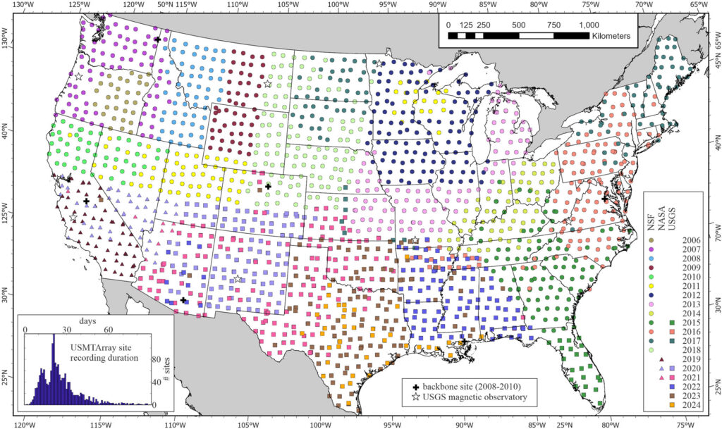
The USMTArray was an ambitious program begun in 2006 under the NSF-funded EarthScope program and completed in June of 2024 under USGS funding. The USMTArray collected long-period MT soundings on a 70-km grid across the contiguous U.S. – totaling more than 1,800 stations – each collected with uniform instrumentation, acquisition parameters, data processing, archiving, and metadata. Funded throughout its 18-year lifetime by three different federal agencies (the NSF, NASA, and USGS working closely with the Incorporated Research Institutions for Seismology and Oregon State University), the data – time series, response functions and metadata – were released incrementally to the public without data embargo or usage restriction.

In broad terms, how was the USMTArray developed?

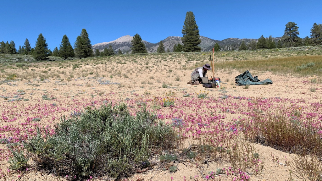
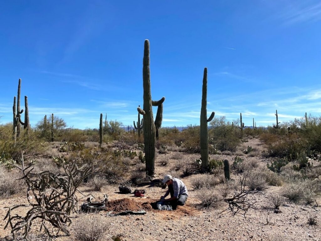
The USMTArray had humble beginnings – being mentioned in early planning documents as having value in understanding subduction zones and characterizing volcanic systems. Funded by NSF in 2003, the MT component of EarthScope was modeled after the much larger seismic component, with a transportable array of instruments to march across the U.S. on a 70-km spaced grid and a backbone array of seven instruments to study deep mantle structure. The USMTArray started off small and before dedicated instruments were even available. In 2006, a pilot study collected the first 30 stations in eastern Oregon using borrowed instruments, while subsequent years expanded what became known as the ‘northwest’ footprint, a 331-sites array completed in 2011 encompassing the Yellowstone-Snake River Plain, the Northern Rocky Mountains, the Cascades magmatic arc, and the northern Basin and Range province. Subsequent footprints in the midcontinent and the eastern U.S. continued to expand coverage.

What were some of the challenges in developing the USMTArray?

The biggest challenge by far was money. Within the EarthScope program, the USMTArray was never funded at the level needed to cover the contiguous U.S. The MT component was instead carried out as a series of footprints in areas deemed most scientifically advantageous. This limitation, however, led to one of the big successes of the USMTArray – active community engagement. Siting workshops held in 2008 and 2013 brought together participants from academia, government, and industry to discuss and prioritize where the array would go next, while a community working group provided scientific and operational guidance throughout the life of the array. The success of the USMTArray was recognized early on by the community governance of the EarthScope facility activities, with the ‘full-48’ concept endorsed in 2009, leading to modest increases in funding and an acceleration of station completions. In 2018, by the end of NSF-sponsored activities, roughly 2/3 of the contiguous U.S. had been covered. Seeing the array to completion, however, required additional funding, a challenge met by NASA (2019-2020) and the USGS (2020-2024), in large part due to recognition of the importance of USMTArray data to space-weather hazards and supported through executive orders in 2016 and 2019.

Another notable challenge that we faced while developing the USMTArray operations was the absence of established data sharing practices within the magnetotelluric community. Indeed, the concept of FAIR data was only introduced in 2016. Back in 2006 when this program commenced, the concepts of open data and systematic data sharing were largely unfamiliar, and no widely adopted, sustainable data formats existed. Available data formats were lacking in flexibility, consistency, and self-descriptive metadata. As the project progressed, our team developed such formats and accompanying databases, which have now reached maturity and are helping to drive more sustainable MT data‑sharing practices internationally.

How has the development of the USMTArray advanced the scientific field?

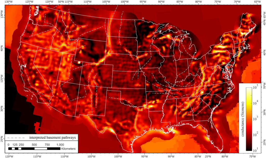
The USMTArray, along with parallel advances in modeling capabilities and increased computational power, ushered in a jump to 3D MT and to interrogating the Earth at regional to national scales. National-scale conductivity models, such as those developed from the USMTArray, now join the ranks of other data sets like magnetic, gravity, and seismic, and are a new lens with which to view the architecture of the North American continent. Numerous contributions to continental architecture and assembly and to understanding active tectonic processes have come from the USMTArray.

The USMTArray also serves as a framework for more detailed studies, allowing Principal Investigators (PIs) to derisk future surveys and industry to investigate anomalous or unexpected structure. Studies of the Cascadia subduction zone and the adjacent magmatic arc and geothermal energy prospectivity studies in the Oregon Cascades and Great Basin have been built upon the USMTArray while new MT surveys along the eastern seaboard are collecting high-resolution MT data to improve space-weather hazard maps over areas identified as particularly at risk from the analysis of USMTArray data.

Beyond the data and models derived from them, the USMTArray has motivated methodological advances, led to an investment in MT instrumentation and open-source software for researchers within the NSF-supported National Geophysical Facility, and served as a model for other regional and continental scale MT experiments.

What are some of the future directions for research in continental scale magnetotellurics?

With completion of the USMTArray, and the 3D conductivity models derived from it, there are numerous avenues for future research. Most models of continental evolution, for example, were developed prior to the advent of this rich data set. Critically evaluating such models in light of this new data set is paramount, and initial studies are already forcing a reexamination of certain paradigms.  

Multi-disciplinary studies incorporating geochronology, geochemistry, and rapidly evolving seismic models is another promising area as is the coupling of geophysical models to geodynamic models to examine the evolution of newly imaged model structure. Similarly, advancements in integrated and joint inversion are promising directions to leverage the wealth of public data sets available at regional to continental scales.  

Geology doesn’t stop at national borders or the land-sea interface – additional opportunities exist for cross-border arrays and onshore/offshore MT studies. Investigation of subduction zone processes and rifted continental margins by their very nature demand an amphibious approach.

On the applied front, resource assessments increasingly are applied at national and even global scales and demand data support at these same scales. Mineral resource assessments, for example, in the U.S., Canada, and Australia are exploring machine learning approaches to map prospectivity for various deposit types and incorporate a range of geophysical data layers to do so. Similarly, geothermal assessments can benefit from the consistent and synoptic data coverage offered by USMTArray data and models.

Finally, on the space-weather hazards front, partnering with power-system engineers to investigate data scale and uncertainty shows promise in generating accurate hazard maps and in improving upon operational, near real-time geoelectric field models. For all these future research directions the USMTArray remains both a framework and a benchmark upon which to build.

—Paul A. Bedrosian (pbedrosian@usgs.gov; 0000-0002-6786-1038), U.S. Geological Survey, United States; Anna Kelbert (anna.kelbert@cfa.harvard.edu; 0000-0003-4395-398X), Center for Astrophysics | Harvard & Smithsonian, United States; Adam Schultz (adam.schultz@oregonstate.edu; 0000-0003-1663-1547), Oregon State University, United States; and Gary D. Egbert (gary.egbert@oregonstate.edu; 0000-0003-1276-8538), Oregon State University, United States

Editor’s Note: It is the policy of AGU Publications to invite the authors of articles published in Reviews of Geophysics to write a summary for Eos Editors’ Vox.

Citation: Bedrosian, P. A., A. Kelbert, A. Schultz, and G. D. Egbert (2026), Mapping the hidden electrical anatomy of a continent, Eos, 107, https://doi.org/10.1029/2026EO265021. Published on 26 May 2026.

This article does not represent the opinion of AGU, Eos, or any of its affiliates. It is solely the opinion of the author(s).

Text © 2026. The authors. CC BY-NC-ND 3.0
Except where otherwise noted, images are subject to copyright. Any reuse without express permission from the copyright owner is prohibited.

Editors’ Vox is a blog from AGU’s Publications Department.

The supply of magma from the Earth’s mantle is a primary source of heat to volcanic arc crust, where the heat is then dissipated through various processes. Much of this magmatic heat is dissipated as heated water, or aqueous fluid.

A new article in Reviews of Geophysics compares 11 different volcanic-arc segments where heat discharge via aqueous fluid has been well-inventoried to better understand the factors that influence this process. Here, we asked the authors to give an overview of heat discharge from volcanic arcs, how scientists measure it, and what questions remain.

Why is it important to study how heat is dissipated from volcanic arcs?

The heat from these magmas matters for geothermal energy, patterns of groundwater flow, and the patterns of volcanic activity at the surface.

Volcanic arcs are the chains of volcanoes on top of subduction zones. They can produce some of Earth’s most explosive and hazardous eruptions. But much of the magma beneath the surface never erupts. Nevertheless, the heat from these magmas—and the simple fact of their existence and abundance—still matters for geothermal energy, patterns of groundwater flow, and the patterns of volcanic activity at the surface.

What are the main modes in which heat is discharged from volcanic arcs?

Heat at volcanic arcs can be carried by magmas, transmitted through the crust conductively, and carried by water seeping slowly through the crust. At the base of the crust, magmas are probably most important, with conduction coming in second. But as magmas move upwards through the crust, some of them solidify and impart their heat to their surroundings where it is transferred by conduction. Within a few kilometers of the surface, fluids seeping through the crust begin to take up all that heat, and so if we can quantify the heat carried by those fluids, we can retrace it to its origins in magmas.

How do scientists measure these different forms of heat loss?

Scientists measure the heat carried by erupting magmas using satellites, or by adding up the erupted masses and making an estimate of how much energy was released by cooling from eruption temperatures to solid igneous rocks at Earth’s surface. Conductive heat flow is measured by drilling holes in the Earth’s crust to see how quickly it gets hotter with depth.

Measuring the heat carried by aqueous fluids in the crust is in some ways the trickiest. One approach is to find all the springs where hot or even slightly warm water is trickling out and measure the temperature and discharge to estimate how much extra heat that water is carrying.

What are the challenges and uncertainties in measuring hydrothermal heat discharge?

One challenge is that many springs are only slightly warmer than you’d expect. There is good data for many hot springs, but there are data tracking these ‘slightly warm’ springs for only a subset of arcs. Another challenge is that warm underground fluids can flow laterally, so you have to try to account for that. This is not an uncertainty in hydrothermal discharge, but one additional big uncertainty for our study, where we were trying to quantify the proportion of magmas that freeze underground versus erupting, is in the estimates of how much magma has actually erupted through time.

What are some of the factors that influence hydrothermal heat loss?

A major goal of our paper is to try to quantify these hidden magmas.

A main factor that influences hydrothermal heat loss is the magmas that solidify underground. This link is the key motivation for our study. A major goal of our paper is to try to quantify these hidden magmas—how much magma needs to intrude the crust beneath the surface to supply the hydrothermal heat fluxes that we observe? The composition of magmas influences how much heat they can release. The depth at which magmas are emplaced also matters, because magmas that intrude the shallow crust eventually cool to lower temperatures than magmas emplaced in the lower crust and therefore release more heat.

What are the remaining questions or knowledge gaps where additional research efforts are needed?

A big outstanding challenge is combining estimates from hydrothermal data of how much magma is coming into the crust – like ours – with other approaches to estimating the same thing. The magmatic systems beneath volcanoes span the crust. At the base of the crust, you have magma supply, sort of like the water main feeding your plumbing system. Despite how fundamental magma supply is, we know remarkably little about it. It’s exciting to think about how the rates of magma supply could vary through time and space and why. Applying a range of techniques—including geophysical imaging, hydrothermal budgets, gas and igneous geochemistry, and petrology—to understand these questions could really be a game changer.

—Benjamin A. Black (bblack@eps.rutgers.edu; 0000-0003-4585-6438), Rutgers University, United States; S. E. Ingebritsen (steve.ingebritsen@gmail.com; 0000-0001-6917-9369), Kyoto University, Japan; and Kazuki Sawayama (sawayama@bep.vgs.kyoto-u.ac.jp; 0000-0001-7988-3739), Kyoto University, Japan

Editor’s Note: It is the policy of AGU Publications to invite the authors of articles published in Reviews of Geophysics to write a summary for Eos Editors’ Vox.

Citation: Black, B. A., S. E. Ingebritsen, and K. Sawayama (2026), Hydrothermal heat flow as a window into subsurface arc magmas, Eos, 107, https://doi.org/10.1029/2026EO265017. Published on 28 April 2026.

This article does not represent the opinion of AGU, Eos, or any of its affiliates. It is solely the opinion of the author(s).

Text © 2026. The authors. CC BY-NC-ND 3.0
Except where otherwise noted, images are subject to copyright. Any reuse without express permission from the copyright owner is prohibited.

Editors’ Vox is a blog from AGU’s Publications Department.

As climate change increases the frequency and intensity of flooding, it’s becoming increasingly important to monitor and predict flood hazards at different scales. A new article in Reviews of Geophysics presents a data-driven performance analysis of various space-based sensors that monitor flood hazards. Here, we asked the lead author to give an overview of satellite-based flood monitoring, the benefits and challenges of using satellite-based sensors, and future space-based projects.

Why is it important to monitor the surface waters on Earth? 

More than half of the world’s population lives within three kilometers of a freshwater body. When seasonal flooding behaves as anticipated, it provides essential nutrient replenishment to soils and crops. However, extreme flooding disturbs the careful balance of freshwater systems and can cause damaging flooding that disrupts livelihoods.

Climate change is making these extremes more frequent and less predictable, while expanding populations in flood-prone areas amplify the human cost. Continuous monitoring of Earth’s surface waters is essential as it helps us anticipate hazards, evaluate risk, and design interventions that protect the people and places most exposed to hydrologic hazards.

What are the benefits of monitoring flood inundation from space compared to other techniques? 

Monitoring flood inundation from space is advantageous due to the wide-scale global coverage that captures important information over large areas. In-situ sensors, such as river gauges, provide valuable data but are limited in spatial coverage and may even fail under significant flood conditions. A single satellite overpass can potentially capture an entire river basin, allowing responders to see where water has spread, which communities are affected, and how the event is evolving.

When did scientists first start using satellites to monitor surface waters?

The value of monitoring surface water from space was first realized in the early 1970s, following the launch of Landsat 1. Soon after launch, it captured imagery of the devastating 1973 Mississippi River floods, producing one of the first flood maps made from space (Figure 1).  By the early 2000s, NASA’s MODIS sensors were providing global coverage at a daily frequency. Today, multiple global flood monitoring systems are in place, including the European Union’s Copernicus Emergency Management Service, which maps floods using Sentinel-1 synthetic aperture radar (SAR), and NOAA’s VIIRS Flood Mapping system.

What are the three types of satellite-based sensors that your review focuses on? 

Our review examines three families. Multispectral (optical and thermal) sensors capture reflected sunlight or emitted heat. Microwave sensors, including SAR, passive microwave radiometers, and GNSS Reflectometry (GNSS-R), can observe through clouds and at night but involve trade-offs between resolution and coverage. Finally, altimetric sensors measure water surface elevation with high precision but only along narrow tracks. Each family has distinct strengths and weaknesses that lend themselves to use in combination for comprehensive flood inundation monitoring.

What are some of the challenges of using satellite-based sensors to monitor flooding?

The fundamental problem is that floods and satellite observations are mismatched in time and space. Optical sensors often capture clouds rather than the floodwater beneath. Cloud-penetrating sensors like SAR can miss flood peaks if their orbital schedule doesn’t align with the event, and dense vegetation can obstruct floodwater from both optical and shorter-wavelength radar. Sensors with high temporal resolution typically deliver data at coarse spatial resolutions, sometimes tens of kilometers per pixel. These trade-offs form what we describe as the “iron triangle” of Earth observation: temporal resolution, spatial resolution, and cost. A sensor can typically be optimized for two, but rarely all three. Occasionally, the timing and conditions of a flood align well with sensors whose strengths are complementary across the iron triangle, yielding the kind of multi-sensor view shown in Figure 2.

What are some upcoming space-based sensor projects that could advance the field of hydrology?

Several are already reshaping the field. NISAR, a joint NASA–ISRO radar satellite launched in 2025, carries an L-band sensor designed to penetrate vegetation canopy, providing new insights into flooding beneath vegetation. Sentinel-1D, launched in late 2025, has restored the Sentinel-1 constellation to full two-satellite capacity, halving the revisit time. Landsat Next, a planned three-satellite constellation with 26 spectral bands and a six-day revisit, would provide valuable hydrologic data at both high temporal and spectral resolutions. However, recent budget pressures have introduced uncertainty about its final scope. Finally, the HydroGNSS mission from ESA will use GNSS-R to monitor hydrologically linked Essential Climate Variables.

—Chloe Campo (S4088633@student.rmit.edu.au; 0009-0007-4259-300X), Royal Melbourne Institute of Technology University: Melbourne, Australia

Editor’s Note: It is the policy of AGU Publications to invite the authors of articles published in Reviews of Geophysics to write a summary for Eos Editors’ Vox.

Citation: Campo, C. (2026), Can any single satellite keep up with the world’s floods?, Eos, 107, https://doi.org/10.1029/2026EO265016. Published on 20 April 2026.

This article does not represent the opinion of AGU, Eos, or any of its affiliates. It is solely the opinion of the author(s).

Text © 2026. The authors. CC BY-NC-ND 3.0
Except where otherwise noted, images are subject to copyright. Any reuse without express permission from the copyright owner is prohibited.

It’s been more than a decade since Michael Gollner and his colleagues first watched a viral YouTube video of a fire tornado fueled by Jim Beam bourbon.

A warehouse in Kentucky had just been struck by lightning, funneling almost a million gallons of the flammable spirit into a nearby retention pond. As the flames whipped across the surface of the water, however, something in the atmospheric stars aligned: The flames coalesced into a towering fire whirl, more commonly known as a fire tornado.

They could, in fact. As Gollner and his collaborators recently reported in Fuel, fire whirls offer the potential to clean up oil spills more quickly and cleanly than existing methods.

Oil spill responses depend on fast, immediate action. After just 24 hours, crude oil naturally absorbs water and begins to sink beneath the waves, wreaking havoc on marine life.

Fire Away

If it’s far from shore, there are few methods other than basically corralling it up and burning it.”

Environmental agencies like the Bureau of Safety and Environmental Enforcement (BSEE) “were very excited about the concept of putting a change to what had been the standard for cleanup since the Exxon Valdez,” Gollner said. “There’s good knowledge, there’s an oil spill conference every year.…But if it’s far from shore, there are few methods other than basically corralling it up and burning it.”

In May 2023, Gollner, Texas A&M aerospace engineering professor Elaine Oran, and two dozen others congregated at the Texas A&M Engineering Extension Service’s (TEEX) Brayton Fire Training Field in collaboration with BSEE. The team erected a trio of 5-meter walls that would channel air flow above a central pool of water, about 3 meters square and 1.2 meters deep, topped by either a 15- or 40-millimeter layer of oil. The scale of the setup was a far cry from traditional fire whirl experiments, which take place mostly in laboratories.

“Everything’s bigger in Texas,” Gollner said.

Why these soot reductions occur is still largely a mystery; probing this question would require building a novel laboratory apparatus to take measurements from within the flame itself, Gollner explained. In the field experiments, meanwhile, one of the fire whirls managed to consume 95% of the available fuel, though the remaining tests extinguished prematurely, lowering the overall rates. Ambient wind conditions on the days of the experiments may also have had some effect.

Summoning a fire whirl in even semi-ideal conditions on the outskirts of College Station, Texas, remains a far simpler task than manifesting one in the thick of a disaster: Towing a three-walled tornado generator onto open water becomes as much a question of marine and naval engineering as of fire science. In the experiment at TEEX, the captive firenado rose to the full length of the 5-meter walls; lower walls could make a floating rig easier to transport, but the resulting mix of oxygen and fuel could actually make subsequent air pollution worse, not better.

Ali Rangwala, a professor of fire protection engineering at Worcester Polytechnic Institute (WPI) who was not involved with the project, also encourages scientific due diligence. A fire whirl “works very well if the boundary conditions are fixed and well-engineered,” he said in an email to Eos, adding that these whirls have yet to be tested on open water with waves and that the required infrastructure may be costly. (Rangwala helped conduct fire whirl experiments with Gollner at WPI but has not maintained a relationship with the project.)

“The honest fact is that this is a disaster-driven field,” Gollner said. One of the largest oil spills in history, the Deepwater Horizon spill, unleashed more than 750 million liters (200 million gallons) into the Gulf of Mexico. That was in 2010. “We haven’t seen a big oil spill for a long time, and interest in it has wavered.…We require a more interdisciplinary team and more testing. Does anyone have the appetite? Unfortunately, I think it will come with time, when we have another accident.”

Blazing a Trail

Gollner stressed the critical value of fundamental research—of lines of inquiry driven by fascination, not just application. What started as a pure appreciation of a natural wonder has the potential to change fields in ways that researchers have yet to imagine.

“Swirling or not, flames are beautiful,” Gollner said. “It is a natural flow tracer. I can see the fluid mechanics and the combustion interacting.…All the physics, all in one: It’s just beautiful.”

—Jonathan Feakins, Science Writer

Citation: Feakins, J. (2026), The fiery tornadoes that could mop up oil spills, Eos, 107, https://doi.org/10.1029/2026EO260158. Published on [DAY MONTH] 2026.

Text © 2026. The authors. CC BY-NC-ND 3.0
Except where otherwise noted, images are subject to copyright. Any reuse without express permission from the copyright owner is prohibited.

Source: Geochemistry, Geophysics, Geosystems

About 600 million years ago, the continents wandered Earth, yet to settle into their current positions. Their locations during the Ediacaran (as this time is called) have been tough for scientists to pin down. Earth’s magnetic field appears to have behaved in erratic ways, and applying standard techniques to calculate the continents’ positions based on records of the magnetic field yields implausible results. In particular, scientists debate the location of an ancient continent called Baltica, which is now part of Europe.

To investigate, Xue et al. traveled to Egersund, Norway, to collect samples of rock that formed during a time when Baltica’s crust was being pulled apart, allowing magma to percolate up from below. As that magma hardened, it recorded snapshots of Earth’s magnetic field, storing information about Baltica’s position in the process.

The results of studying these samples revealed a much more complex picture of the ancient rocks than the scientists initially envisioned. The rocks contained a messy mix of at least six magnetic signals. Several appeared to have formed when more modern geological processes altered the original rocks. Three distinct signals may have survived from the Ediacaran period, two of which diverge from the most plausible Ediacaran signal, which places Baltica near the equator. These conflicting signals further support the idea that Earth’s magnetic field was behaving strangely at the time, adding new complexity to an already puzzling picture.

On the basis of the new results, the researchers place the Egersund paleomagnetic pole at 20.8°N, 89.0°E during the Ediacaran—which diverges from previous results—and suggest that Baltica was located near the equator, adjacent to the ancient continent Laurentia, but rotated slightly clockwise relative to previous reconstructions. The study demonstrates the convoluted nature of the magnetic signals preserved in ancient rocks and the importance of dissecting those records into their constituent components. Doing so, the researchers suggest, can shed new light on the enigmatic behavior of Earth’s magnetic field during the Ediacaran. (Geochemistry, Geophysics, Geosystems, https://doi.org/10.1029/2025GC012730, 2026)

—Saima May Sidik (@saimamay.bsky.social), Science Writer

Citation: Sidik, S. M. (2026), Where was Baltica 616 million years ago?, Eos, 107, https://doi.org/10.1029/2026EO260124. Published on 5 2026.

Text © 2026. AGU. CC BY-NC-ND 3.0
Except where otherwise noted, images are subject to copyright. Any reuse without express permission from the copyright owner is prohibited.

Source: Geochemistry, Geophysics, Geosystems

This is an authorized translation of an Eos article. 本文是Eos文章的授权翻译。

大约 6 亿年前，各大洲在地球上漂移，尚未最终定格在现在的位置。在埃迪卡拉纪时期，各大洲的位置对于科学家来说一直难以确定。地球的磁场似乎表现得异常不稳定，而利用标准方法根据磁场记录来计算大陆位置的做法却得出了一些难以置信的结果。尤其是，科学家们对一块名为波罗的大陆的古老大陆的位置存在争议，这块大陆如今是欧洲的一部分。

为了探究这一问题，Xue等人前往挪威埃格尔松德，采集了波罗的大陆地壳被撕裂、岩浆从下方涌出时形成的岩石样本。随着这些岩浆冷却凝固，它们记录了地球磁场的瞬时变化，并在此过程中存储了有关波罗的大陆位置的信息。

对这些样本的研究结果揭示了远比科学家们最初设想的更为复杂的古代岩石图景。这些岩石中至少包含了六种不同的磁信号，构成了一幅复杂的混合图景。其中一些信号似乎是在更现代的地质过程改变原始岩石时形成的。埃迪卡拉纪时期可能保存了三种不同的信号，其中两种与将波罗的板块置于赤道附近的最合理的埃迪卡拉纪信号相悖。这些相互矛盾的信号进一步支持了地球磁场在当时异常活动的观点，使原本就扑朔迷离的图景更加复杂。

基于新的研究结果，研究人员将埃迪卡拉纪时期埃格尔松德古地磁极的位置确定在北纬20.8°、东经89.0°——这与之前的研究结果有所不同——并提出波罗的板块当时位于赤道附近，毗邻古老的劳伦古陆，但相对于之前的重建结果，其位置略有顺时针旋转。这项研究表明，保存在古代岩石中的磁信号极其复杂，并凸显了将这些记录分解成各个组成部分的重要性。研究人员认为，这样做可以为埃迪卡拉纪时期地球磁场的神秘行为提供新的线索。(Geochemistry, Geophysics, Geosystems, https://doi.org/10.1029/2025GC012730, 2026)

—科学撰稿人Saima May Sidik (@saimamay.bsky.social)

This translation was made by Wiley. 本文翻译由Wiley提供。

Read this article on WeChat. 在微信上分享本文。

Text © 2026. AGU. CC BY-NC-ND 3.0
Except where otherwise noted, images are subject to copyright. Any reuse without express permission from the copyright owner is prohibited.

Albert Einstein postulated in his 1905 theory of special relativity that the speed of light in a vacuum is constant. Ever since, that’s been one of the fundamental assumptions of physics.

Now Enbang Li, a physicist at the University of Wollongong in Australia, has challenged this idea by building a machine he says is capable of detecting changes in the speed of light as it crosses Earth’s surface. The findings suggest that light is, in fact, sped up by gravity, which could have implications for Earth science applications ranging from climate monitoring to mineral resource exploration.

An Old Conundrum

The idea that light is influenced by gravity is not new. Einstein’s ideas, which were further developed with his theory of general relativity in 1915, predicted massive objects in space would bend light with their gravitational grab. This theory was famously proven in 1919 when two independent teams measured starlight passing a solar eclipse at two different points on Earth’s surface and found the results matched Einstein’s predictions.

This bending of light’s path, according to general relativity, is achieved by a warping of the space-time fabric. Under this scenario, the speed of light remains constant—it just has to travel farther as it navigates the warped space-time around celestial bodies, so to a distant observer, it appears to have been slowed.

But what if light doesn’t navigate warped space-time and actually is slowed down or sped up by the gravity of large objects?

Li pointed out that Einstein himself was not always convinced the speed of light was constant. In 1911, he wrote a paper postulating that light speed changed depending on the gravity of objects it passed by. However, “when he published his general theory,” said Li, “he just abandoned this model.”

If the movement of light can be affected by gravity, Li reasoned, it might be possible to detect variations in its speed on a local level—such as an elevator shaft in a building on the campus of the University of Wollongong.

Raising the Big Issues

Gravity on Earth varies locally, depending on altitude, underground density, and topography. Gravity at the top of a tall building, for example, is measurably weaker than it is at the bottom.

With these variations in mind, Li installed an experiment in an elevator. It consisted of a coil of fiber-optic cable that if stretched out in one direction, would be 10 kilometers (6.2 miles) long. Laser beams were fired through the cables and then reflected back, thus traveling 20 kilometers (12.4 miles) before reaching an ultrafast photodetector. An oscilloscope measured the time it took for the beam to travel that distance. The experiment was run at the top of the shaft and at the bottom.

The biggest challenge, Li said, was filtering out all the surrounding environmental “noise,” such as changing temperature and humidity, electromagnetic disturbance, and building vibrations. Li designed a temperature control system, and the experiment was sealed in an enclosure with electromagnetic shielding to isolate air flows. Li ran the experiment and found light moved minutely faster at the bottom of the shaft than at the top.

Gravity Sensing on the Go

Next, Li took his research a step further by building a small, portable machine he claims can detect changes in the speed of light as it nears more gravitationally dense objects.

In this second experiment, Li positioned a moveable 72-kilogram (159-pound) weight near the machine. Light, he found, moved faster when the weight was near the machine than when it was farther away.

The results, which were published in Scientific Reports, are consistent with the variable speed of light model Einstein proposed in 1911, although Li’s preliminary results are much larger than that model predicts.

If proven, the findings would present a fundamental challenge to our understanding of both general and special relativity.

In the world of Earth sciences, they could lead to greatly improved gravity-sensing technologies. Because of their sensitivity to changes in mass, gravity sensors are used to map the seafloor and to locate underground mineral reserves. Gravity sensing can also improve our understanding of Earth’s climate as variations in the gravity field can be linked to factors like changes in ice mass and shifts in groundwater.

Currently, gravimeters are vulnerable to vibrations and movement, whereas Li’s machine, which has no moving parts, could even be used on board a plane or submarine.

“A Striking Claim”

Chris Stevens, a numerical relativist with the University of Canterbury in New Zealand, called the work “intriguing and ambitious.” While Stevens, who was not involved in the research, said that Li’s work is “well founded,” he noted that any observable effects of gravity on light on Earth would be “extraordinarily small” and therefore these results must be treated with caution.

“In my own research on observable gravitational phenomena,” he explained, “I usually require a few black holes colliding somewhere in the universe. Separating genuine gravitational signatures from environmental and instrumental noise will therefore be exceptionally demanding.”

“The work is exciting because it pushes precision photonic measurement techniques into a regime where relativistic effects may become practically useful for geophysics and sensing applications.”

Stevens said the implications of Li’s research, if validated, would be far-reaching. “The work is exciting because it pushes precision photonic measurement techniques into a regime where relativistic effects may become practically useful for geophysics and sensing applications.”

John Norton, an historian of physics at the University of Pittsburgh who was also not involved in the research, called the findings a “striking claim.” He was, however, skeptical of them, saying “if there is a coupling between light and gravity of magnitude greater than general relativity predicts, it is hard to see how the 1919 eclipse test and later studies of gravitational lensing would not have found it.”

Li acknowledged there is a long way to go before his device finds everyday use. Disentangling the intricacies of space and time, he said, is a vast challenge. “In physics, people still say gravity is a mystery. Light is another mystery. So if you put these two mysteries together, that’s going to be a giant mystery.”

—Bill Morris, Science Writer

Citation: Morris, B. (2026), How Einstein’s lost theory could help us find minerals, Eos, 107, https://doi.org/10.1029/2026EO260189. Published on 12 June 2026.

Text © 2026. The authors. CC BY-NC-ND 3.0
Except where otherwise noted, images are subject to copyright. Any reuse without express permission from the copyright owner is prohibited.

Researchers have found that Earth’s underlying crust in the Turkana Rift region has been significantly thinned, presaging Africa’s eventual breakup—and with that finding, the researchers offer a new perspective on Turkana’s fossil record of human evolution.

Editors’ Vox is a blog from AGU’s Publications Department.

Mesoscale and submesoscale ocean processes influence ocean circulation, air-sea fluxes, ecosystem variability, and transport of materials. A new article in Reviews of Geophysics examines how these fine-scale processes shape the Indian Ocean, an ocean basin with unique monsoon behavior and a disproportionate impact on global climate. Here, we asked the authors to explain what mesoscale and submesoscale processes are, the techniques and challenges of observing and modeling fine-scale processes, and how biogeochemical cycles and climate change interact with these processes.

In simple terms, what are mesoscale and submesoscale processes?

Mesoscale processes pertain to oceanic features such as eddies and fronts, which
typically span a range of approximately 10 to 100 kilometers and can persist from
weeks to months. Submesoscale processes are of an even smaller scale, ranging
between approximately 100 meters and 10 kilometers, and evolve rapidly within a time frame of hours to days. These encompass sharp fronts, filaments, and small vortices.

Mesoscale processes account for more than 80% of the total kinetic energy. Submesoscale motions are of particular significance as they generate robust vertical movements that establish a connection between the surface ocean and deeper layers. As elaborated in our review, mesoscale and submesoscale processes function as a crucial link between large-scale ocean circulation and small-scale turbulence, facilitating the transfer of energy across different scales and regulating the distribution of heat, salt, and nutrients throughout the ocean.

Why is it important to understand how fine-scale processes operate in the Indian Ocean?

The Indian Ocean has a disproportionate influence on global climate.

The Indian Ocean has a disproportionate influence on global climate. It absorbs over a quarter of the ocean’s net heat gain and directly affects the environment and food security of nearly one-third of the world’s population. Unlike other ocean basins, the Indian Ocean is uniquely shaped by seasonally reversing monsoon winds and is strongly coupled with climate modes like the Indian Ocean Dipole and the Madden- Julian Oscillation. Mesoscale and submesoscale variability in this region modulates biogeochemical cycles, air-sea fluxes, and even large-scale energy balance. As our review highlights, understanding these fine-scale dynamics is essential for improving predictions of monsoon rainfall, tropical cyclone behavior, and long-term climate change.

How do scientists study mesoscale and submesoscale ocean processes?

Scientists employ a combination of field measurements, satellite observations, and numerical models, all of which were summarized in our review. In-situ observations serve as the foundation for mesoscale and submesoscale processes in the ocean. They encompass research cruises, moored arrays such as the RAMA network, Argo profiling floats, and autonomous platforms. The in-situ observations capture the three-dimensional structures and multiple variables during mesoscale and submesoscale processes.

Satellite altimetry has long been the principal tool for observing mesoscale eddies. However, the newly launched Surface Water and Ocean Topography (SWOT) mission is revolutionary, as it offers sea surface height measurements at an unprecedented resolution, enabling the direct observation of submesoscale features for the first time.

High-resolution regional models with grid spacings of a few kilometers or less enable researchers to simulate these processes and test dynamical theories under controlled conditions.

What are some of the challenges in observing and modeling these processes?

In our review paper, we tackled the challenges in observations by adhering to four principles, namely high-resolution (more observations in a relatively small region), synchrony (observations conducted at the same time), persistence (observations for a long time), and interdisciplinary (observations of multiple ocean properties). These principles are anticipated to offer valuable guidance for future observational endeavors to surmount the corresponding challenges.

Modeling also poses difficulties. Even state-of-the-art climate models are unable to explicitly resolve submesoscale processes. Consequently, their effects have to be approximated via parameterizations. The development of accurate parameterizations continues to be an active area of research. Moreover, as the model resolution improves, the widely employed hydrostatic approximation may lose its validity, necessitating more intricate non-hydrostatic formulations. Data assimilation for such rapidly evolving features presents a particularly arduous challenge.

How do fine-scale processes interact with biogeochemical cycles in the Indian Ocean?

Mesoscale and submesoscale motions exert a strong regulatory influence on biogeochemical cycling.

Mesoscale and submesoscale motions exert a strong regulatory influence on biogeochemical cycling through the control of nutrient supply to the sunlit upper ocean. Cyclonic eddies elevate nutrient-rich deep waters into the euphotic zone, thereby promoting phytoplankton blooms. In contrast, anticyclonic eddies typically suppress surface productivity by deepening the mixed layer.

In the Arabian Sea, eddies and filaments can contribute up to 70% of the nutrients that support the monsoon-driven biological bloom. These fine-scale dynamics also have an impact on carbon dioxide exchange; mesoscale variability accounts for approximately 40% of the CO₂ flux variability in the western Arabian Sea. Moreover, eddies modulate oxygen minimum zones in the Arabian Sea and Bay of Bengal, where low oxygen levels have a profound effect on marine ecosystems.

How is climate change expected to influence these fine-scale processes in the Indian Ocean?

With the continuous progression of climate change, alterations in upper-ocean stratification, propelled by warming and modified freshwater inputs, are anticipated to transform the conditions giving rise to fine-scale instabilities. High-resolution climate model simulations suggest that in a warming global scenario, the eddy-active region associated with the Agulhas Current system may shift westward and poleward. This shift is correlated with the intensification of Agulhas leakage, which refers to the transport of warm Indian Ocean water into the Atlantic. These changes could exert far-reaching effects on global ocean circulation.

Warming is augmenting the frequency and intensity of marine heatwaves in the Indian Ocean.

Moreover, warming is augmenting the frequency and intensity of marine heatwaves in the Indian Ocean. These heatwaves disrupt vertical mixing and nutrient supply, thereby having cascading impacts on biological productivity. Nevertheless, substantial uncertainties persist in quantifying these long-term responses.

In general, there are two-way interactions between climate change and fine-scale processes. Alterations in one component will induce changes in the other, and the former will be subject to feedback from the latter.

What are the remaining questions or knowledge gaps where additional research is needed?

Our review reveals several key priorities. In the short term, specialized multi-scale observational campaigns are acutely required, especially in regions with insufficient sampling, to capture the three-dimensional structure and rapid evolution of submesoscale features. Additionally, a more in-depth understanding is needed regarding how eddies interact with barrier layers—regions characterized by strong salinity stratification that are unique to the northern Indian Ocean—and how these interactions regulate air-sea fluxes and marine heatwaves.

Longer-term challenges encompass integrating fine-scale dynamics into climate models and refining submesoscale parameterizations. Emerging tools from artificial intelligence and machine learning hold potential for representing unresolved processes and enhancing data assimilation. Finally, considering the logistical and financial requirements of fine-scale ocean research, sustained international collaboration will be indispensable.

—Lei Zhou (zhoulei1588@sjtu.edu.cn, 0000-0002-0433-3991) Shanghai Jiao Tong University, China; Dongxiao Wang (dxwang@mail.sysu.edu.cn, 0000-0001-8778-2188) Sun Yat-Sen University School of Marine Sciences, South China Sea Institute of Oceanology, China; Lin Wang (wanglin58@mail.sysu.edu.cn, 0009-0003-1062-5207) Sun Yat-Sen University, China; and Chunhua Qiu (qiuchh3@mail.sysu.edu.cn, 0000-0001-9684-6067)  Sun Yat-sen University School of Marine Sciences, China

Editor’s Note: It is the policy of AGU Publications to invite the authors of articles published in Reviews of Geophysics to write a summary for Eos Editors’ Vox.

Citation: Zhou, L., D. Wang, L. Wang, and C. Qiu (2026), Small-scale Indian Ocean dynamics underpin marine ecology and climate, Eos, 107, https://doi.org/10.1029/2026EO265025. Published on 4 June 2026.

This article does not represent the opinion of AGU, Eos, or any of its affiliates. It is solely the opinion of the author(s).

Text © 2026. The authors. CC BY-NC-ND 3.0
Except where otherwise noted, images are subject to copyright. Any reuse without express permission from the copyright owner is prohibited.

Tiny saltwater channels have a big influence on sea ice.

Sea ice typically includes pockets or channels of brine that allow salt water to flow vertically through the ice. When those channels align neatly, they need to make up only about 5% of the ice volume before the water can flow. But in more disordered, granular ice, salt water starts to flow only when the brine channels take up more space—roughly 10% of the ice volume, according to a new study published in Scientific Reports.

“If we’re trying to find predictive models about how these ice cores are responding under climate change, it’s going to be necessary to take into account these structural and microstructural conditions.”

This higher threshold could slow the drainage of surface melt ponds, as well as the transport of nutrients to microbial communities inside the ice.

“If we’re trying to find predictive models about how these ice cores are responding under climate change, it’s going to be necessary to take into account these structural and microstructural conditions,” said Stephen Ackley, a sea ice researcher at the University of Texas at San Antonio who was not involved in the study.

Disorderly Constructs

As seawater freezes, it forms a mixture of ice crystals and brine. In calm conditions, the ice slowly grows into long, parallel crystals separated by orderly brine channels. This columnar sea ice is common in the Arctic, and its properties have been widely used in sea ice models.

But in choppy waves or when the ice’s snow-covered surface floods and refreezes, new ice can’t grow into these ordered columns. Instead, it forms small, randomly oriented grains separated by more complex pores containing brine and gases. Called granular ice, this form is more common in Antarctica but is becoming increasingly prevalent in the Arctic as temperatures rise and ice cover thins.

“It’s the sequel we’ve been waiting decades for.”

In 1998, University of Utah mathematician Kenneth Golden established the first estimate of the point at which the brine channels are connected enough to allow water to flow in columnar ice, called the percolation threshold. The new work, also led by Golden, extends a similar analysis to granular sea ice.

“It’s the sequel we’ve been waiting decades for,” said Don Perovich, a sea ice researcher at Dartmouth who was not involved in the new work.

To quantify the percolation threshold for granular ice, Golden and his colleagues collected sea ice samples during two expeditions off the eastern coast of Antarctica in 2007 and 2012. They measured how quickly water moved through the brine channels in the ice. After the 2012 expedition, they also mapped the arrangement of ice crystals within the ice blocks to correlate those permeability measurements with the microscale structure of the ice.

The finding that in granular ice, about twice as much of the ice volume needs to be brine for water to flow compared to columnar ice suggests that brine channels within granular ice are much less interconnected.

With the higher threshold, “you have to reassess all these models, anything that relies on fluid flow through sea ice,” if granular ice is present, said Golden. Granular ice will require warmer or saltier conditions to leave enough brine in the ice structure to meet the percolation threshold and allow water to flow vertically.

For example, the new value could influence models of how meltwater ponds behave atop an underlying ice sheet. If meltwater ponds form above a base of granular sea ice, those ponds will require warmer temperatures before they start draining than melt ponds on columnar ice will.

If these melt ponds remain on the surface longer waiting for those warmer temperatures, they could lower the albedo, or reflectivity, of the ice sheet. That could cause the ice sheet to absorb more heat, leading to a feedback loop that could accelerate melting.

The higher percolation threshold could also affect algae that lives within the ice. Ice algae make up an important food source for krill and crustaceans, which in turn become food for fish, penguins, and whales. Algae rely on water flowing through the ice to deliver nutrients. Because granular ice requires warmer temperatures for that flow to start, it could affect the depth at which algae can live inside the ice, Golden said.

Percolation Consideration

Still, experts say more data are needed to establish percolation thresholds across both Arctic and Antarctic ice. The size of the grains in granular ice can vary substantially at different temperatures, under different formation conditions, and between the poles. Larger grains could lower the percolation threshold, allowing water to flow even when the ice contains much less than 10% brine by volume, said Sønke Maus, a scientist studying ice microstructure at the Norwegian University of Science and Technology who was not involved in the study.

“The data that we have at the moment for the granular sea ice is sparse,” Maus said. “You need a big campaign to collect such data.”

Golden said that in future work he also plans to develop models to compute the electromagnetic properties of both columnar and granular sea ice. Knowing these properties can help scientists determine the thickness and age of an ice sheet from satellite data.

—Skyler Ware (@skylerdware), Science Writer

Citation: Ware, S. (2026), Changes in sea ice microstructure could affect climate models, Eos, 107, https://doi.org/10.1029/2026EO260164. Published on 20 May 2026.

Text © 2026. The authors. CC BY-NC-ND 3.0
Except where otherwise noted, images are subject to copyright. Any reuse without express permission from the copyright owner is prohibited.

Editors’ Vox is a blog from AGU’s Publications Department.

Ensuring the sustainability of water resources and ecosystems in a changing world requires a thorough understanding of how water moves through Earth’s Critical Zone, a dynamic interface where air, water, soil, plants, and rocks interact. Researchers can track and model this movement of water using naturally occurring markers or “tracers.”

A recent article in Reviews of Geophysics explores the latest advancements in tracer-aided mixing models and how they can help us to better understand the Critical Zone. Here, we asked the authors to give an overview of the Critical Zone, how tracer-aided mixing modeling works, and future directions for research.

What is the Critical Zone (CZ)?

The Critical Zone is Earth’s “living skin”—the dynamic layer where the atmosphere, hydrosphere, biosphere, and lithosphere interact. It stretches from the top of the vegetation canopy and, in cold regions, from the surface of snowpacks and glaciers, down through soils and into the deeper aquifers. It encompasses lakes, streams, and wetlands at the surface, and extends beyond the soil layer to underlying groundwater aquifers. It is where rainfall, snowmelt and glacier melt become soil moisture, where plants take up water and return it to the atmosphere, where aquifers get recharged, and where streamflow is generated. In short, the Critical Zone is where most processes that sustain terrestrial life and freshwater resources unfold.

Why is it important to understand how water moves through the Critical Zone?

Virtually every freshwater resource we rely on (e.g., drinking water, irrigation) passes through the Critical Zone.

Virtually every freshwater resource we rely on (e.g., drinking water, irrigation) passes through the Critical Zone at some point. Global warming, land-use changes, and intensifying water demand emerging from rapid urbanization and changes in agriculture are reshaping how water is stored and released within the Critical Zone, often in ways we cannot yet predict. Understanding how much water is stored within the Critical Zone, how this water is both recharged from rainfall and snowmelt and eventually discharged into streams, and the timescale of these dynamic processes is essential for protecting ecosystems, safeguarding water supplies, and adapting to a changing climate.

How would you explain a tracer-aided mixing model to a non-specialist?

Imagine mixing a glass of orange juice with a glass of apple juice, and trying afterwards to work out how much of each went into the glass. If the juices had distinctive “fingerprints” (imagine its color, sugar content, or a specific chemical) and these fingerprints primarily changed because of the mixing of these two juices, you can then measure the fingerprint in the final mixture and back-calculate the proportion of its distinct sources.

Tracer-aided mixing models work in a similar way but can track the entire water cycle. Different water sources (e.g., rainfall, snowmelt, glacier melt, soil water, groundwater) can have distinct “fingerprints” in a naturally occurring tracer, such as stable isotopes of water or specific dissolved elements. By measuring these fingerprints in the streamwater or groundwater and in its potential sources for example, hydrologists can estimate how much each source contributed to the streamwater or groundwater.

What are some of the most significant and exciting recent advances in tracer-aided mixing models?

Classical mixing models relied on demanding assumptions: that all water sources can be identified and sampled, and that their signatures were distinct and constant in time. Much of the recent progress has been about relaxing these assumptions.

Bayesian approaches now estimate full probability distributions and provide a more realistic picture of uncertainty. Methods like Convex Hull End-Member Mixing Analysis (CHEMMA) use machine learning to infer the distinct sources directly from data, while ensemble hydrograph separation exploits tracer fluctuations over time, thereby making un-mixing feasible even when multiple sources have overlapping signatures. Perhaps the most conceptually novel advance is end-member splitting, which flips the question from “where does streamflow come from?” to “where does precipitation go?”

Alongside these modeling advances, there have been immense advances in how tracers are measured. Portable laser and mass spectrometers now enable high-frequency, in-situ tracer measurements which allows us to capture critical hydrological events such as storms and snowmelt in near-real time.

What are stable water isotope tracers and what are their advantages?

Stable water isotopes are naturally occurring non-radioactive atoms of hydrogen and oxygen that make up a water molecule but have slightly different molecular masses. The two stable isotopes widely used in hydrology are 2H (deuterium) and 18O (oxygen-18). Because these isotopes are part of the water molecule itself, they directly travel with the water molecule. Their key advantages are: (1) they are conservative, meaning they do not react chemically as water moves through soils and aquifers, and (2) they carry distinct signatures resulting from climatic variables such as air temperature.

These properties make stable water isotopes the most versatile and widely used tracer in Critical Zone hydrology.

Consequently, in the European Alps, winter precipitation has a different isotopic signature than summer precipitation because winters are cooler than summers. Other hydrological processes such as evaporation and sublimation leave a recognizable fingerprint on the remaining water, thereby allowing us to estimate how much evaporation or sublimation occurred. Stable water isotopes can be measured in essentially every water compartment, from atmospheric vapor and precipitation to snowpack, plant xylem, soil water, streams, and groundwater. Together, these properties make stable water isotopes the most versatile and widely used tracer in Critical Zone hydrology.

What are the current limitations of tracer-aided mixing models?

Despite their power, mixing models still face many constraints. End-member signatures vary in space and time, are sometimes too similar to distinguish, and some sources may be overlooked entirely. Non-conservative tracers such as nitrate or sulfate can react with their environment along their journey, thereby biasing results if these reactions are not explicitly accounted for.

Sampling is another major bottleneck. Capturing the spatial heterogeneity of soils, snowpacks, and groundwater requires a lot of measurements that are often logistically or financially prohibitive, especially in remote regions. Many of the newer, more powerful tracers such as noble gases or stable isotopes of trace elements, can only be analyzed by a handful of specialized laboratories. As a result, global coverage remains highly uneven, with key regions such as the Arctic and the global South still under-sampled.

What are some of the major unsolved questions and where is more research needed?

There are several fronts where more research is needed. Source signatures are not static, and methods that explicitly capture their variability in time are still underdeveloped. Embedding tracers within global Earth System Models would, in theory, enable more accurate assessment of hydrological partitioning e.g., how rainfall, snowmelt, and glacier melt are split between sublimation, evapotranspiration, groundwater, and streamflow. These will directly inform more robust climate projections, but this remains technically demanding.

Expanding data coverage in under-sampled regions is critical, and citizen science and low-cost sensors may help. Machine learning is a promising approach for uncovering non-linear relationships and gap-filling sparse datasets, but requires training data that often do not yet exist. Greater interdisciplinary integration, e.g., combining tracers with remote sensing, ecological indicators, and biogeochemical data, could yield a more holistic view of the Critical Zone. Finally, the field would benefit from shared protocols and open data practices to enhance progress.

—Andrea L. Popp (andrea.popp@smhi.se; 0000-0003-3911-8105), Swedish Meteorological and Hydrological Institute, Sweden; Harsh Beria (hberia@ethz.ch; 0000-0003-2597-9449), ETH Zurich, Switzerland

Editor’s Note: It is the policy of AGU Publications to invite the authors of articles published in Reviews of Geophysics to write a summary for Eos Editors’ Vox.

Citation: Popp, A. L., and H. Beria (2026), Tracing water’s hidden journey through the Earth’s living skin, Eos, 107, https://doi.org/10.1029/2026EO265019. Published on 13 May 2026.

This article does not represent the opinion of AGU, Eos, or any of its affiliates. It is solely the opinion of the author(s).

Text © 2026. The authors. CC BY-NC-ND 3.0
Except where otherwise noted, images are subject to copyright. Any reuse without express permission from the copyright owner is prohibited.

Editors’ Vox is a blog from AGU’s Publications Department.

Explosive volcanic eruptions inject gases and ash into the atmosphere, posing major hazards for human health, infrastructure, and aviation. A new article in Reviews of Geophysics examines recent advances in estimating Eruption Source Parameters (ESPs), the key conditions at the volcanic vent that are a necessity for modeling the behavior of volcanic plumes. Here, we asked the authors to explain what ESPs are, what technologies are used to observe eruptions, and which scientific challenges and future research directions remain for improving volcanic plume monitoring and modeling.

In simple terms, what are Eruption Source Parameters?

Eruption Source Parameters (ESPs) describe the key conditions at the volcanic vent during an eruption.

Eruption Source Parameters (ESPs) describe the key conditions at the volcanic vent during an eruption, such as the mass eruption rate, exit velocity, temperature, and particle size distribution. These parameters define how material is injected into the atmosphere and are essential inputs for models that simulate plume rise and subsequent dispersal of volcanic gases and ash in the atmosphere. In simple terms, ESPs represent the boundary conditions that control the behavior of volcanic plumes. Because they cannot usually be measured during an eruption, they must be estimated from indirect observations and models, which introduces significant uncertainty.

Why is it important to understand how volcanic ash and gases disperse after an eruption?

Volcanic ash and gases can travel long distances and affect aviation safety, human health, infrastructure, and even climate. Fine ash particles are particularly hazardous for aircrafts, while ash fallout can disrupt communities and critical services on the ground. Gas emissions may also impact air quality and alter the atmospheric radiative budget. Understanding volcanic dispersion is therefore essential for forecasting the movement of volcanic clouds and issuing timely warnings. Reliable forecasts support risk mitigation strategies and enable more effective responses by civil protection agencies and aviation authorities.

What technologies are used to observe volcanic plumes?

Volcanic plumes are observed using a combination of satellite, ground-based, and, more rarely, airborne measurements. Satellite observations are crucial for tracking ash and gas clouds over large spatial scales and in near real time. Ground-based instruments, such as radar, cameras, and infrasound sensors, provide detailed information on plume dynamics close to the source. Increasingly, these observations are integrated with numerical models to infer eruption conditions. The combination of multiple data streams is essential for constraining ESPs and improving the reliability of plume simulations.

What are some of the recent advances in estimating Eruption Source Parameters?

Recent advances have focused on combining observations with numerical models to better constrain ESPs. Multi-sensor approaches, data inversion techniques, and improved plume models have significantly enhanced our ability to estimate eruption rates and plume dynamics. At the same time, high-resolution computational fluid dynamics (CFD) simulations provide deeper insights into the complex fluid dynamic processes governing plume behavior. However, these models are computationally expensive and unsuitable for real-time applications, highlighting the need for approaches that bridge the gap between physical realism and operational efficiency.

What strategies do you propose in your review to improve Eruption Source Parameters estimation?

A central contribution of this review is the proposal of a new class of operational models for volcanic plumes.

A central contribution of this review is the proposal of a new class of operational models for volcanic plumes. These models integrate the physical realism of high-fidelity CFD simulations with the efficiency of simplified models used in forecasting. In particular, the review highlights the potential of artificial intelligence and machine learning techniques to “learn” from CFD results and optimally calibrate the key variables controlling plume dynamics. This hybrid approach allows complex physical processes to be represented in a computationally efficient framework, making it suitable for real-time applications while retaining improved accuracy.

How does improved volcanic plume monitoring lead to more effective volcanic hazard assessment?

Improved monitoring leads to more accurate estimates of ESPs, which directly translate into better forecasts of plume rise and ash dispersion. This reduces uncertainty in hazard assessments and supports more reliable decision-making. For example, more accurate forecasts can help aviation authorities minimize disruptions while maintaining safety and enable civil protection agencies to issue targeted warnings. Ultimately, better integration of observations and models enhances the capacity to respond effectively during eruptions and to mitigate their societal and economic impacts.

What are the remaining questions or knowledge gaps where additional research is needed?

Further research is needed to improve the coupling between observations, physics-based models, and data-driven approaches.

Despite progress, significant challenges remain. ESPs are still difficult to constrain in real time, and uncertainties in both observations and models propagate into forecasts. The integration of diverse data sources is not yet fully optimized, and different estimation methods can yield inconsistent results. Further research is needed to improve the coupling between observations, physics-based models, and data-driven approaches. In particular, developing robust hybrid frameworks that combine CFD, simplified models, and machine learning represents a key direction for advancing both scientific understanding and operational forecasting.

—Antonio Costa (antonio.costa@ingv.it, 0000-0002-4987-6471), Istituto Nazionale di Geofisica e Vulcanologia, Italy

Editor’s Note: It is the policy of AGU Publications to invite the authors of articles published in Reviews of Geophysics to write a summary for Eos Editors’ Vox.

Citation: Costa, A. (2026), From volcanic vents to safer skies, Eos, 107, https://doi.org/10.1029/2026EO265022. Published on 27 May 2026.

This article does not represent the opinion of AGU, Eos, or any of its affiliates. It is solely the opinion of the author(s).

Text © 2026. The authors. CC BY-NC-ND 3.0
Except where otherwise noted, images are subject to copyright. Any reuse without express permission from the copyright owner is prohibited.